Kinetic Simulation of Nonequilibrium Kelvin-Helmholtz Instability
Lin Chuan-Dong1, †, Luo Kai H.1, 2, ‡, Gan Yan-Biao3, Liu Zhi-Peng4
1Center for Combustion Energy, Key Laboratory for Thermal Science and Power Engineering of Ministry of Education, Department of Energy and Power Engineering, Tsinghua University, Beijing 100084, China
2Department of Mechanical Engineering, University College London, Torrington Place, London WC1E 7JE, UK
3North China Institute of Aerospace Engineering, Langfang 065000, China
4Department of Physics, School of Science, Tianjin Chengjian University, Tianjin 300384, China


† Corresponding author. E-mail: chuandonglin@163.com K.Luo@ucl.ac.uk

Abstract
Abstract

The recently developed discrete Boltzmann method (DBM), which is based on a set of uniform linear evolution equations and has high parallel efficiency, is employed to investigate the dynamic nonequilibrium process of Kelvin-Helmholtz instability (KHI). It is found that, the relaxation time always strengthens the global nonequilibrium (GNE), entropy of mixing, and free enthalpy of mixing. Specifically, as a combined effect of physical gradients and nonequilibrium area, the GNE intensity first increases but decreases during the whole life-cycle of KHI. The growth rate of entropy of mixing shows firstly reducing, then increasing, and finally decreasing trends during the KHI process. The trend of the free enthalpy of mixing is opposite to that of the entropy of mixing. Detailed explanations are: (i) Initially, binary diffusion smooths quickly the sharp gradient in the mole fraction, which results in a steeply decreasing mixing rate. (ii) Afterwards, the mixing process is significantly promoted by the increasing length of material interface in the evolution of the KHI. (iii) As physical gradients are smoothed due to the binary diffusion and dissipation, the mixing rate reduces and approaches zero in the final stage. Moreover, with the increasing Atwood number, the global strength of viscous stresses on the heavy (light) medium reduces (increases), because the heavy (light) medium has a relatively small (large) velocity change. Furthermore, for a smaller Atwood number, the peaks of nonequilibrium manifestations emerge earlier, the entropy of mixing and free enthalpy of mixing change faster, because the KHI initiates a higher growth rate.

1 Introduction

The Kelvin-Helmholtz instability (KHI), named after Lord Kelvin and Hermann von Helmholtz, arises at the perturbed interface between fluids in shear motion, and leads to the formation of vortices and turbulence.[12] KHI phenomena are ubiquitous in nature and engineering.[35] Examples include waves on a windblown ocean or sand dune, swirling cloud billows, the stream structure of solar corona, the helical wave motion in ionized comet tails, the Great Red Spot in Jupiters atmosphere, the Eagle Nebula in astrophysics, the reacting mixing layers in combustion, and the ignition in inertial confinement fusion. The KHI is one of the most fundamental and famous instabilities in fluid dynamics, and it is often coupled with other instabilities, such as Rayleigh-Taylor instability,[67] Richtmyer-Meshkov instability,[89] etc. Hence, due to its great importance, the KHI has been studied extensively in experimental,[7,1011] theoretical,[6] and numerical fields.[1213]

Particularly, with the rapidly improving computational facilities and algorithms, numerical simulation has achieved more and more successes in scientific research and engineering application. Roughly speaking, there are three kinds of numerical methods: microscopic,[1415] mesoscopic,[1316] and macroscopic approaches,[17] respectively. Microscopic models, such as molecular dynamics[14] and direct simulation Monte Carlo,[15] describe the location and motion of particles in detail, but usually demand too high computational cost. Macroscopic schemes, such as direct numerical simulation, large eddy simulation, and Reynolds-averaged Navier-Stokes (NS) equations, improve computational efficiency significantly, but lose various thermodynamic nonequilibrium information which plays an essential role in interfacial dynamics. To reach a compromise between the computational cost and physical fidelity, a promising method is mesoscopic kinetic modelling based on the Boltzmann equation.

In the last three decades, the kinetic-based lattice Boltzmann method (LBM)[1820] has been developed and become a powerful tool for investigating coherent structures and detailed nonlinear dynamics of complex flows, including the KHI.[2126] However, most researchers were more likely to take the LBM as a numerical solver of hydrodynamic equations rather than a kinetic model of nonequilibrium systems. Therefore, little consideration has been given to the kinetic nature of related systems. As a novel variant of the LBM, the discrete Boltzmann method (DBM) overcomes the above issue.[2732] It has the capability of simulating the dynamic process of KHI properly by incorporating essential nonequilibrium effects.[2732] In 2011, Gan et al. proposed a kinetic model for compressible systems and studied the KHI under the influence of velocity and density gradients.[27] This model recovers the Euler equations in the continuum limit, and works for single-component flows. In 2016, Lin et al. developed a DBM for two-component systems.[31] This model recovers the compressible NS equations when the Knudsen number approaches zero,[31] and provides more accurate physical information than the former.[27] In the current work, we employ the two-component DBM to study the nonequilibrium process of KHI.

This paper is organized as follows: In Sec. 2, we introduce the DBM that provides detailed nonequilibrium information and high parallel efficiency. In Sec. 3, we use the DBM to study the nonequilibrium effects, entropy of mixing, and free enthalpy of mixing in the KHI process. Finally, conclusions are given in Sec. 4.

2 Discrete Boltzmann Model

The discrete Boltzmann equations with single collision term take the form,
where t indicates the time, the discrete velocity, σ the fluid species, ( ) the discrete (equilibrium) distribution function, and τσ the relaxation time. Note that, for a two-component system (σ = A and B), the relaxation of the two species should be equal in order to ensure the local momentum conservation, i.e., .[33] The relaxation time is specified as a function of species concentration in Ref. [33]. For simplicity, it is given a constant value here. Additionally, two-dimensional simulations are carried out in the present study, although the formulation can be easily extended to three dimensions. We adopt the second Runge-Kutta scheme for the time derivative and the second order nonoscillatory and nonfree-parameter dissipative finite difference scheme[34] for the space derivatives in Eq. (1).

The discrete velocity reads, , with , . The suffix i indicates the direction of the discrete velocity, and k indicates the k-th group of the particle velocities whose speed is vk. To be specific, and . To ensure the simulation robustness, an optimal choice is . Figure 1 delineates the sketch of the discrete-velocity-model.[35]

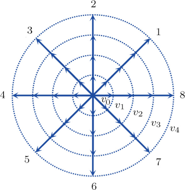
Fig. 1. Sketch of the discrete-velocity-model.

The expression of reads,
with the flow speed u, and , where mσ represents the molar mass, T the temperature. The weighting coefficients are,

where the suffixes
The mole concentration, mass density, flow velocity, and energy of species σ are calculated as below


The mole concentration, mass density, flow velocity and temperature of the mixing are , , , and , respectively. Mathematically, the coupling between the Boltzmann equations for the two species is achieved achieved via the flow speed and temperature T which enter the expression of the equilibrium distribution functions in Eq. (2). In this way, the cross-collisions of species A and B exchange physical information between them.

It is easy to prove that the DBM could recover the NS equations in the hydrodynamic limit.[31] Moreover, the DBM can be employed to measure the following nonequilibrium manifestations,


with the central velocity, . The second-order tensor corresponds to the viscous stress tensor, with the unit vector in the α direction. The vector is related to the heat flux. and are higher order nonequilibrium quantities beyond traditional NS models. To roughly estimate the “degree of nonequilibrium”, we introduce the following four condensed measures,
The value of is used to measure the strength of the viscous stress; indicates the intensity of the heat flux; and represent the degrees of and , respectively. Physically, , , , and are zero only in equilibrium. Otherwise, they are nonzero, and become larger as the fluid system departs further from its local equilibrium.

Theoretically, similar to the standard LBM, the DBM has the outstanding merits of simplicity for programming and high parallel efficiency, because the discrete Boltzmann equation is uniformly linear and all the information transfer in DBM is local in time and space. However, the parallel efficiency of our DBM has never been demonstrated in a numerical way. To this end, we conduct simulations using parallel programming based on the Message-Passing Interface standard. Calculations are carried out on the supercomputer ARCHER. Table 1 exhibits the parallel efficiency. Eight tests are performed using the number of processing cores, Np = 1 × 1, 2 × 2, 4 × 4, 8 × 8, 16 × 16, 32 × 32, 64 × 64, and 128 × 128, respectively. The mesh is chosen as . The other parameters are identical to those for Fig. 4. After 8000 iterative steps, the running time is , , , , , , , and seconds, respectively. Define the parallel efficiency as , with . Then the efficiency is 100%, 95.4%, 85.7%, 85.6%, 84.9%, 83.8%, 83.5%, and 82.0% for the eight tests, respectively. It is evident that the parallel efficiency of the DBM is quite high.

Table 1.

Parallel efficiency study of the DBM.

.

To validate its capability of describing the interaction between two species, this DBM is used to simulate binary diffusion. Initially, the mole concentration is described by the following step function, and , where the suffixes L and R index the left and right parts, respectively. The temperature is T = 1, the velocity , the molecular mass mσ = 1, the relaxation time τ = 10−3, the temporal step Δ t = 10−5, the spatial step , the mesh grid . Figure 2 displays the mole fraction of species A at three time instants. Symbols are for DBM results, and solid lines for the analytical solution
where is the initial mole fraction difference, and χ = 10−3 the diffusion coefficient. We can find a satisfying agreement between the two sets of results.

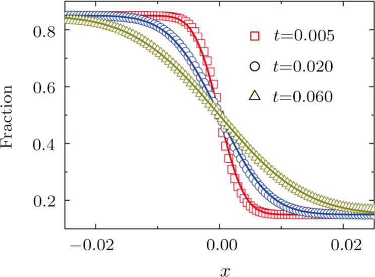
Fig. 2. Mole fractions YA in the binary diffusion at time instants: t = 0.005, 0.020, and 0.060, respectively. Symbols stand for DBM simulation results, and solid lines for the corresponding analytical solutions.
3 Simulation and Investigation

In this section, let us focus on the KHI. The initial field configuration is delineated in Fig. 3. The left part is occupied by species A with an upward velocity and a mole concentration , the right part is full of B with a downward velocity and a mole concentration . Between them is a perturbed interface with a transition layer. Mathematically,
where Dρ (Du) represents the width of density (velocity) transition layer, x0 denotes the averaged x position of the cosine-shaped interface, W and k are the perturbation amplitude and wave number, respectively. The pressure p is equal at the two sides of the interface. The two species have an identical velocity and temperature at the same location. The length and width of the physical domain are Lx = 1.5 and Ly = 0.5, respectively. The parameters are chosen as , , , , , , , , , . Furthermore, boundary conditions are as follows: the inflow/outflow (zero gradient) boundary conditions in the x direction, the periodic boundary conditions in the y direction. In addition, all quantities are expressed in nondimensional forms, i.e., the widely accepted LB units,[27] in this work.

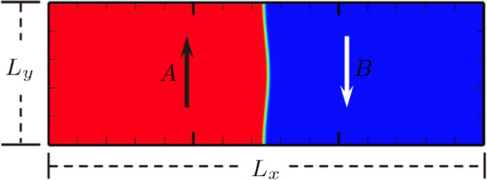
Fig. 3. Field configuration.
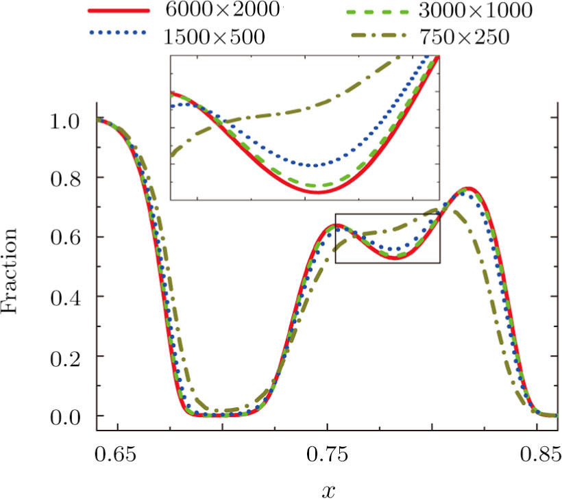
3.1 Grid Convergence Test

Grid convergence is one of the most important issues in numerical simulations. To verify the validity of the simulation, a grid convergence test is firstly carried out using various grids: , 1500 × 500, 3000 × 1000, and 6000 × 2000, respectively. The time step is , the relaxation time , the molar mass mA = 3, and mB = 1. Figure 4 delineates the molar fraction YA (= nA/n) along the line y = Ly/2 at the time t = 1. As one can see, with increasing mesh grids, the numerical errors become smaller and smaller. The differences between simulations with grids 6000 × 2000 and 3000 × 1000 are small enough. Taking account of both accuracy and efficiency, we carry out this simulation on the gird 3000 × 1000.

Fig. 4. Grid convergence test: molar fraction of species A along the line y = Ly/2 at the time t = 1. The solid, dashed, dotted, and dot-dashed lines denote the mesh grids
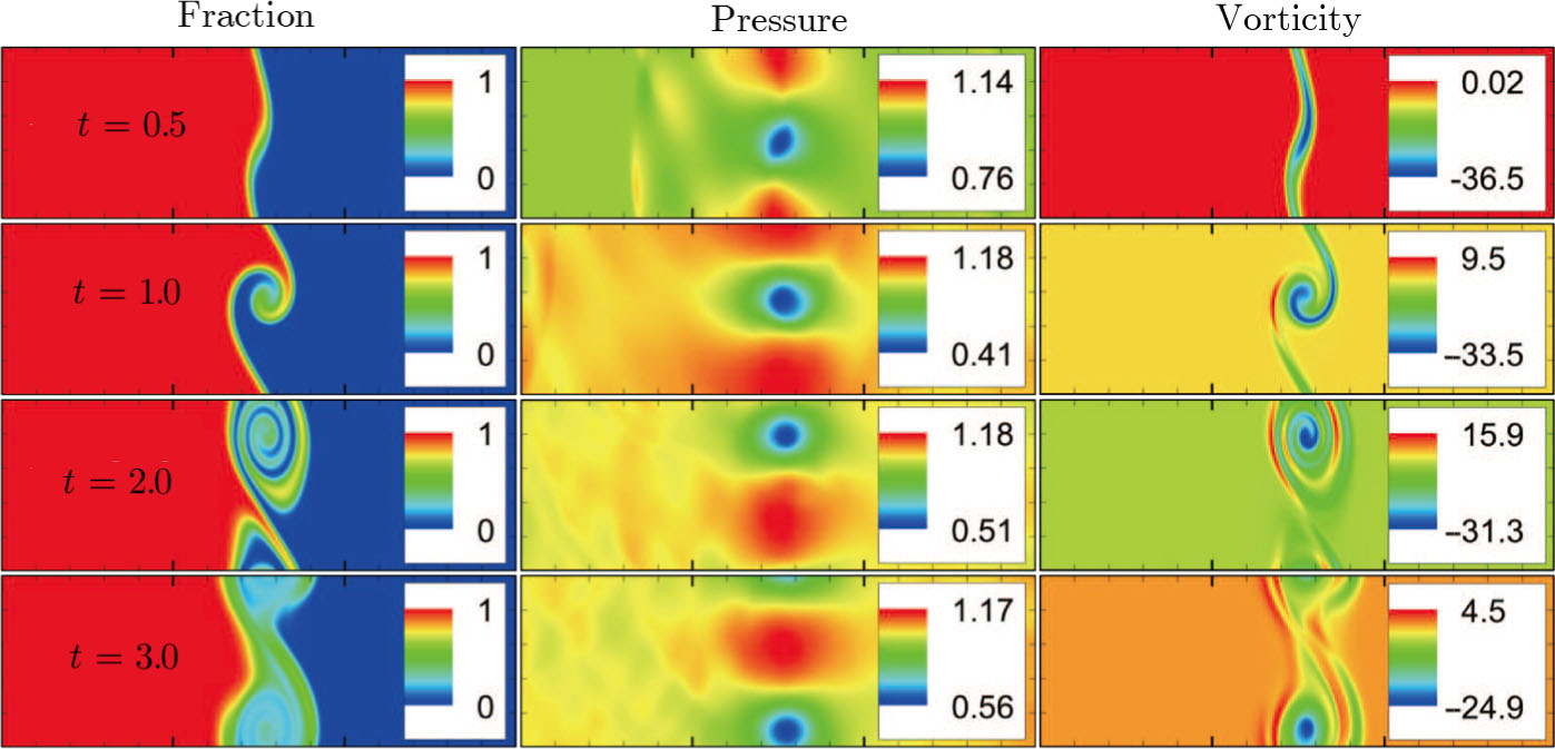
 , 3000 × 1000, 1500 × 500, and 750 × 250, respectively. The inset enlarges the outlined rectangular region.

Figure 5 depicts the molar fraction YA, pressure p (= nT), and vorticity at time instants t = 0.5, 1.0, 2.0, and 3.0, respectively. It is evident that the perturbed interface begins to wiggle due to the velocity shear at t = 0.5. After the initial linear growth stage, a rolled-up vortex emerges around the interface at t = 1.0. Then, at t = 2.0, a larger vortex is observed in the snapshot. At t = 3.0, the thickening interfacial layer indicates that KHI promotes the mixing and penetrating of the miscible fluid components. Comparing pressure contours with vorticity, we can find that the minimum pressure is located at the vortex center, and the maximum pressure is at the position where two opposite direction flows encounter each other. The flow field varies with space and time. In fact, the pressure gradient offers the centripetal force required by the rotating flows. Moreover, the interface is continuous and smooth, as shown in Fig. 5. The coherent structures demonstrate that the DBM has a good ability of capturing interface deformation.

Fig. 5. Contours of physical quantities at time instants t = 0.5, 1.0, 2.0, and 3.0, respectively. The leftmost, middle, and rightmost columns show the snapshots of the molar fraction of A, pressure, and vorticity, respectively.
3.2 Nonequilibrium Effects

As an initial application, we preliminarily study two kinds of nonequilibrium effects, and , in the evolution of KHI. To give an intuitive impression, Fig. 6 depicts the contours of them at the moment t = 2.0. The values of and are greater than zero around the vortex where the shear is significant, while they are close to zero far away from the interface where the velocity difference is low. Meanwhile, values of and are large at the contact between the two media, while they approach zero where the interaction between the fluids is weak.

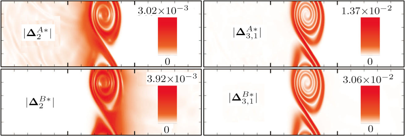
Fig. 6. Contours of nonequilibrium quantities, and , at the moment .

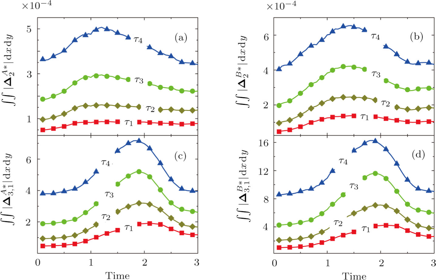
To investigate the influence of relaxation time on the nonequilibrium KHI, we conduct four runs with various relaxation times, , , , and , respectively. Let us define the Reynolds number as , where the characteristic density is , the characteristic velocity , the characteristic length , the dynamic viscosity . Correspondingly, Re = 3750, 1875, 937.5, and 468.75, for the four runs, respectively. Taking into account of both numerical accuracy and computational efficiency, we chose the spatial step as , , , and , respectively. And the temporal step is , , , and , respectively.

Figure 7 plots the evolution of nonequilibrium quantities and , respectively, where the integral is extended over all physical space . Actually, and indicate the global nonequilibrium effect (GNE) of species σ in the physical region from two different points of view. stands for the global strength of the viscous stress, while represents the global intensity of the heat flux. The lines with squares, diamonds, circles, and triangles stand for the relaxation times τ1, τ2, τ3, and τ4, respectively. It is evident that the GNEs become stronger for larger relaxation times. The evolution of GNE shows firstly increasing then decreasing trends. and do not reach their peaks simultaneously, and reaches the maximum earlier than . Physically, there are competitive mechanisms in the evolution of GNEs. The GNE is associated with the local nonequilibrium effect and the nonequilibrium area. On the one hand, the interface is lengthened with the development of the vortex. The increasing interface enhances the GNEs. On the other hand, the interface is widened in the process of the binary diffusion and thermal conductivity, hence the physical gradients become smooth. The reducing physical gradients weaken the local nonequilibrium effects.

Fig. 7. Evolution of nonequilibrium quantities with various relaxation times: (squares), (diamonds), (circles), and (triangles), respectively. (a) . (b) . (c) . (d) .
3.3 Entropy of Mixing

In thermodynamics, entropy of mixing is part of the increasing entropy when separate systems with different components contact and mix, before the establishment of a thermodynamic equilibrium state. The statistical concept of randomness is utilized for statistical mechanical explanation of the entropy of mixing. Mathematically, the entropy of mixing per unit volume takes the form,
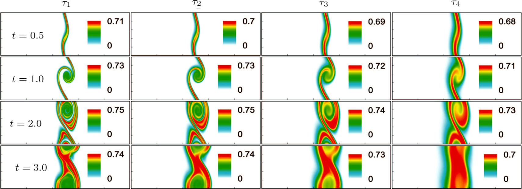
where Yσ is the molar fraction of species σ. The entropy of mixing is a typical thermodynamic nonequilibrium variable. It indicates the mixing extent and nonequilibrium process in various miscible fluid systems.

Figure 8 illustrates the snapshots of entropy of mixing in the evolution of KHI. The four columns, from left to right, correspond to cases with relaxation times τ1, τ2, τ3, and τ4, respectively. The four rows, from top to bottom, correspond to the time instants t = 0.5, 1.0, 2.0, and 3.0, respectively. It is clear in each column that the mixing area increases in the evolution of KHI. The rolled-up vortex lengthens the interface and promotes the mixing process. Meanwhile, it can be found in every row that the mixing area is larger for a larger relaxation time, because the diffusion coefficient, which enhances the mixing process is proportional to the relaxation time.[36]

Fig. 8. Contours of the entropy of mixing at time instants t = 0.5, 1.0, 2.0, and 3.0, respectively. The four columns, from left to right, correspond to the relaxation times , , , and , respectively.

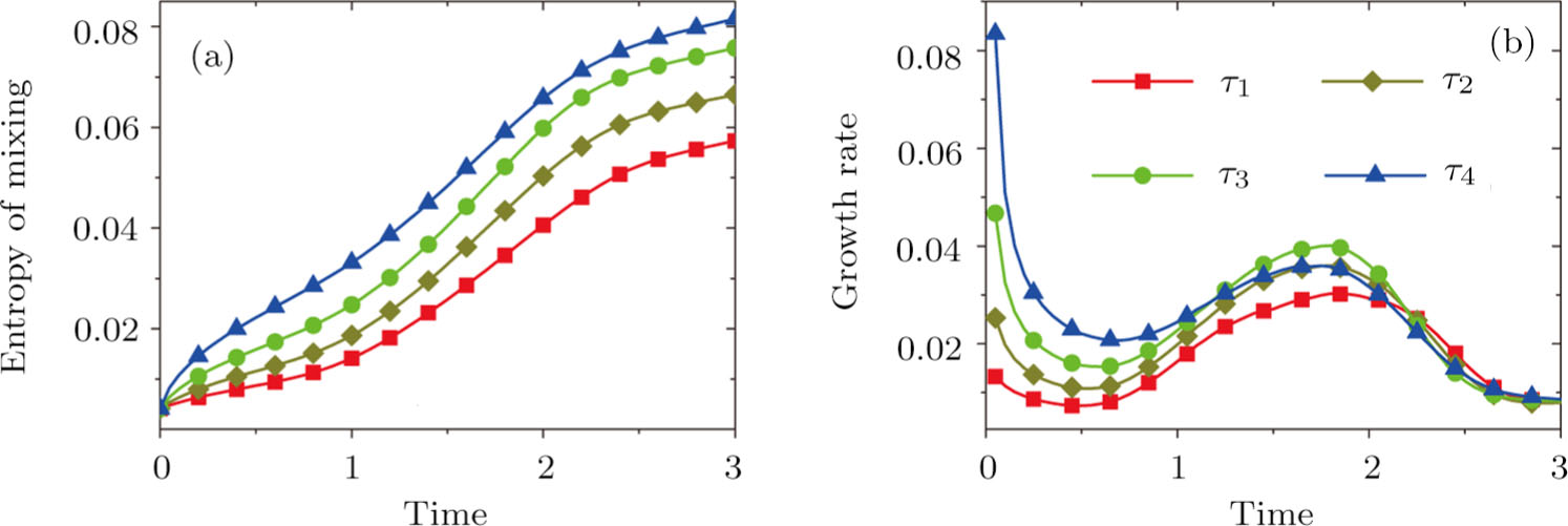
For the purpose of a quantitative study, we probe the temporal evolution of entropy of mixing with various relaxation times. Figure 9(a) shows , where the integral is extended over all physical region, and Fig. 9(b) plots its growth rate. Obviously, in Fig. 9(a), the entropy of mixing is higher for a larger relaxation time, which is consistent with Fig. 8. Moreover, it is interesting to see in Fig. 9(b) that the evolution of its growth rate shows three trends, i.e., firstly reducing, then increasing, and finally decreasing trends. Physically, there are competitive mechanisms in the evolution of the entropy of mixing. (i) The binary diffusion is fast when the gradient of molar fraction is sharp. The transition layer of the initial interface is relatively narrow, hence the diffusion and mixing is relatively fast. The mixing rate reduces with the increasing width of the transition layer in the early stage. (ii) The mixing process is promoted by the increasing length of material interface with the development of the vortex. In the evolution of KHI, the interface becomes longer and longer, hence the mixing rate increases in the second stage. (iii) With the ongoing diffusion, the material interface becomes wide and the gradients are smoothed. The mixing rate reduces and begins to approach zero, when the gradient becomes smaller and smaller around the vortex, in the final stage. It is of interest to find that the fast diffusion promotes the mixing process directly and initially, but slows the mixing rate indirectly and finally, in the dynamic process of KHI.

Fig. 9. Evolution of entropy of mixing and its growth rate with various relaxation times: (squares), (diamonds), (circles), and (triangles), respectively.
3.4 Free Enthalpy of Mixing

In thermodynamics, free enthalpy of mixing is another interesting thermodynamic nonequilibrium variable. Let us introduce Gibbs free enthalpy of mixing per unit volume as below,
Note that since and . In other words, free enthalpy of mixing is always nonpositive, and it is opposite to entropy of mixing that is nonnegative. Mathematically, .

Figure 10 depicts the fields of free enthalpy of mixing and temperature at time instants t = 0.5, 1.0, 2.0, and 3.0, respectively. The case corresponds to the first column in Fig. 8 with the relaxation time . In order to make a clear comparison to the entropy of mixing, the minus free enthalpy of mixing is shown. Since the free enthalpy of mixing is the function of the entropy of mixing and temperature, the contours of temperature are plotted aside. A comparison between Figs. 8 and 10 gives two points. On the one hand, the entropy of mixing and minus free enthalpy of mixing exhibit similar contours, as both of them are located at the interface between the two species. On the other hand, the entropy of mixing and minus free enthalpy of mixing show some different values due to the spatio-temporal variation of temperature in the evolution of KHI.

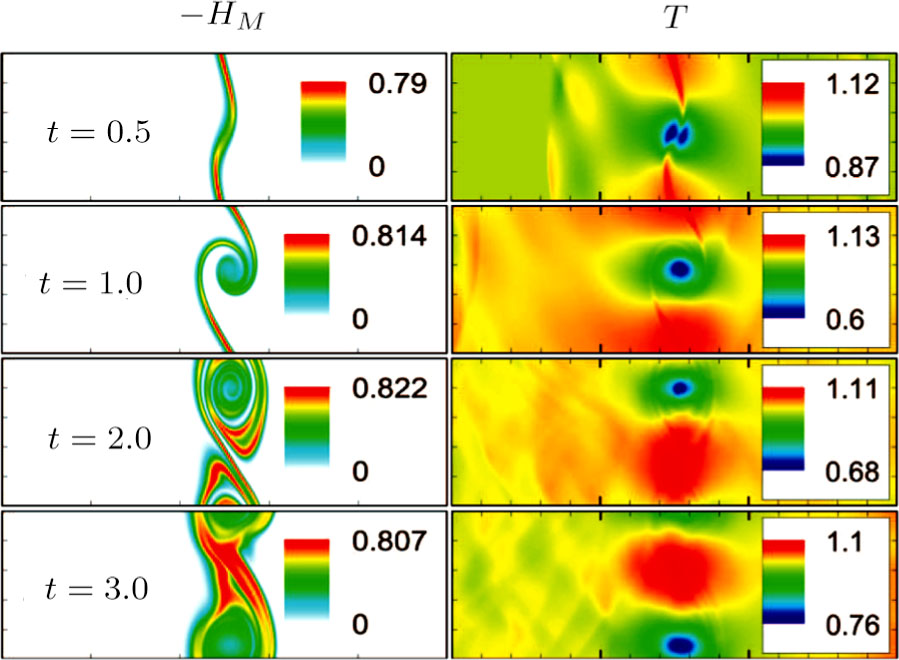
Fig. 10. Contours of minus free enthalpy of mixing ( ) and temperature (T) with the relaxation time τ = 10−4 at time instants t = 0.5, 1.0, 2.0, and 3.0, respectively.

Figure 11(a) plots , where the integral is extended over all physical region, and Fig. 11(b) illustrates its growth rate. In contrast to the entropy of mixing, the free enthalpy of mixing is lower for a larger relaxation time, and its growth rate displays three different trends, i.e., firstly increasing, then decreasing, and finally increasing trends. The tendency of the growth rate of free enthalpy of mixing is opposite to that of entropy of mixing. The physical mechanisms for the free enthalpy of mixing are identical with that for the entropy of mixing.

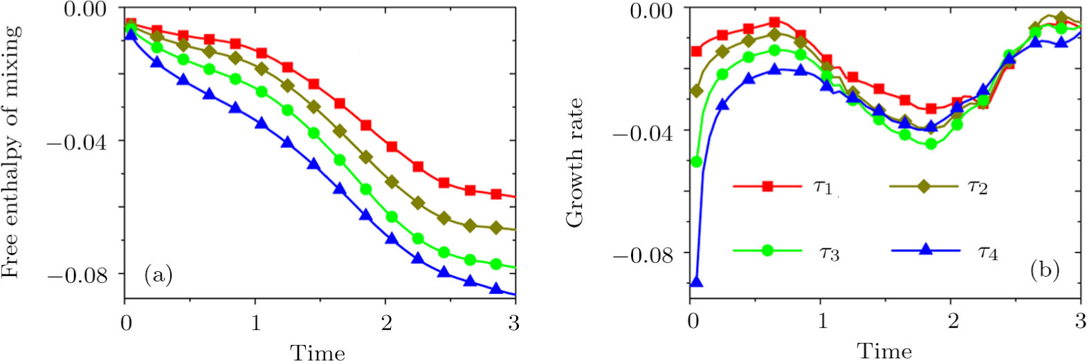
Fig. 11. Evolution of the free enthalpy of mixing and its growth rate with various relaxation times: (squares), (diamonds), (circles), and (triangles), respectively.
3.5 Atwood Number

Atwood number is an important parameter that affects the growth of KH instability. It is defined as
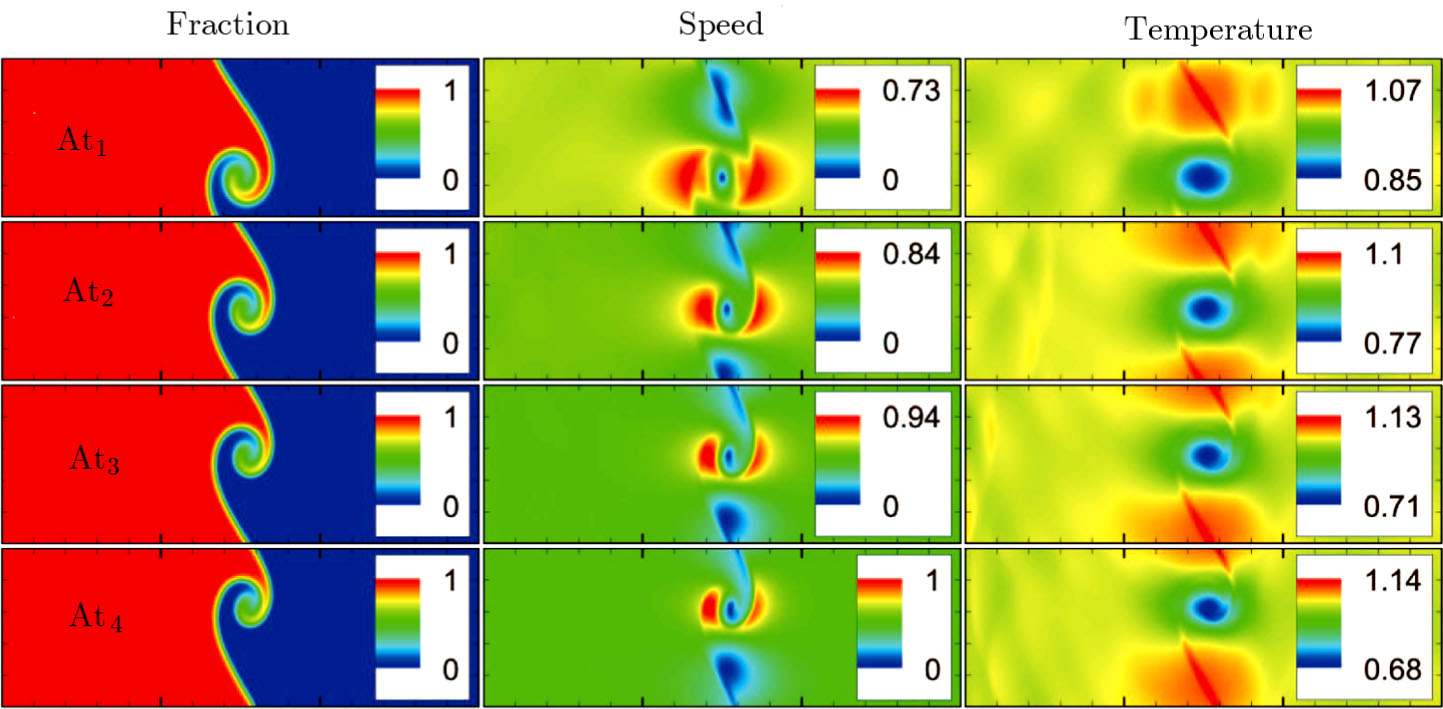
with and nσ = 1 in this section. Let us consider four cases, i.e., mA=1, 2, 3, and 4, with fixed mB=1. The corresponding Atwood numbers are At1 = 0, At2 = 1/3, At3 = 1/2, and At4 = 3/5, respectively. The other parameters are the same as those in Fig. 5.

Figure 12 depicts the snapshots of the molar fraction YA, the speed , and the temperature T at time t = 1 with various Atwood numbers. We can find an upward movement in the vortex center with the increasing Atwood numbers. Physically, the average flow velocity in the y direction, uy, is zero around the interface for the case mA = mB, and it increases with the increasing mass ratio of species A to B, i.e., . Hence the vortex goes up as the flow speed uy increases with the increasing Atwood numbers. Moreover, it is clear in the first column that the vortex becomes wider in the x direction for a smaller Atwood number. The second column shows that the maximum flow speed increases with the increasing Atwood number. It can be obtained from the first and second columns that the light medium B has larger speed than the heavy one A around the vortex. Finally, the third column shows that, with the increasing Atwood number, the maximum temperature increases and the minimum temperature reduces. It is seen from the first and third columns that the minimum temperature is located at the vortex center, while the maximum temperature is located at the interface where the conversion from the shear kinetic energy to the internal energy is intense. In sum, the vortex has a smaller area, the light medium has faster speed, and the temperature has sharper gradients for a larger Atwood number.

Fig. 12. Contours of physical quantities at time t = 1. The leftmost, middle, and rightmost most columns are for the molar fraction of A, flow speed, and temperature, respectively. The four rows from top to bottom correspond to Atwood numbers At1 = 0, At2 = 1/3, At3 = 1/2, and At4 = 3/5, respectively.

Figure 13 exhibits the evolution of nonequilibrium quantities with various Atwood numbers. Figure 13(a) shows that, for species A, the global strength of viscous stress, , is smaller for a larger Atwood number. On the contrary, for species B, the global strength of the viscous stress, , increases with the increasing Atwood number, as shown in Fig. 13(b). Physically, with the increasing mass ratio of species A to B, the flow velocity of the heavy medium A has a relatively small change, while the flow velocity of the light one B has a relatively large change, during an interval. In addition, Fig. 13(c) shows that the global intensity of the heat flux, , decreases with the increasing Atwood number. While in Fig. 13(d), the peak of the global intensity of the heat flux, , is similarly high for different Atwood numbers. Because, mathematically, is roughly inversely proportional to mσ.[32] Furthermore, for a larger Atwood number, the peaks of either or emerge later, because the amplitude of the perturbed interface grows more slowly.[6]

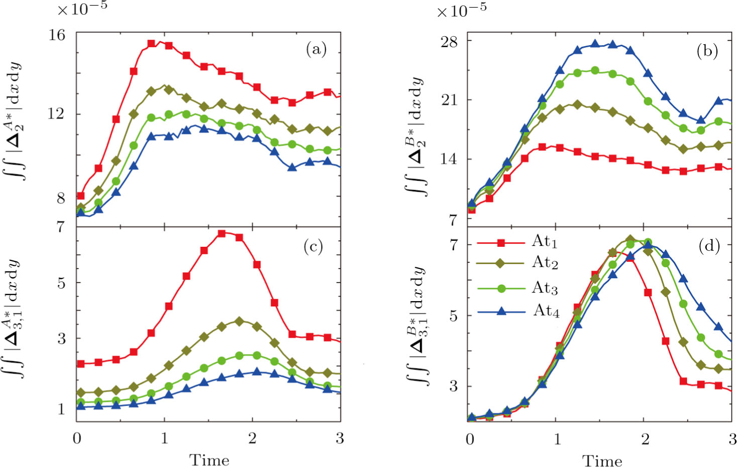
Fig. 13. Evolution of nonequilibrium quantities with various Atwood numbers: At1 = 0 (squares), At2 = 1/3 (diamonds), At3 = 1/2 (circles), and At4 = 3/5 (triangles), respectively. (a)
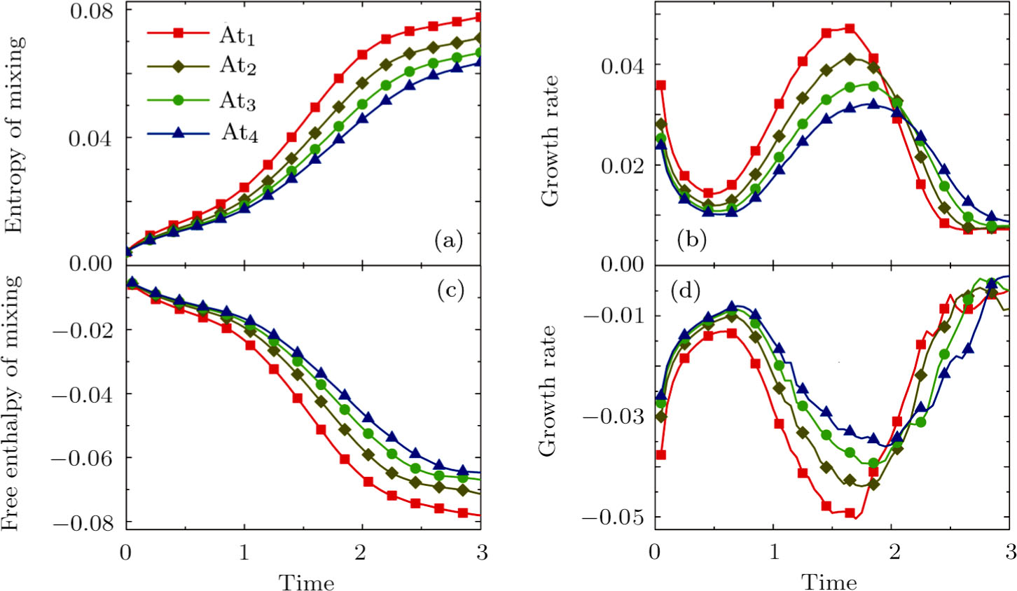
 , (b) , (c) , (d) .

Figure 14 illustrates the evolution of entropy of mixing, free enthalpy of mixing, and their growth rates with the Atwood number: At1 = 0 (squares), At2 = 1/3 (diamonds), At3 = 1/2 (circles), and At4 = 3/5 (triangles), respectively. It is evident in Fig. 14(a) that the entropy of mixing is lower for a larger Atwood number. Figure 14(b) shows that, for each Atwood number, the growth rate of entropy of mixing has three trends, i.e., firstly reducing, then increasing, and finally decreasing trends. In contrast, as shown in Figs. 14(c) and 14(d), the free enthalpy of mixing is higher for a larger Atwood number, and its growth rate shows firstly increasing, then reducing, and finally increasing trends. The trough (peak) in Fig. 14(b) and the peak (trough) in Fig. 14(d) take place almost simultaneously. Both the trough and peak emerge earlier for a smaller Atwood number in either Fig. 14(b) or Fig. 14(d). Because the growth rate of the perturbed interface is higher and the mixing area is wider for a smaller Atwood number, as shown in Fig. 12.

Fig. 14. (a) Entropy of mixing and (b) its growth rate, (c) free enthalpy of mixing and (d) its growth rate, with the Atwood number: At1 = 0 (squares), At2 = 1/3 (diamonds), At3 = 1/2 (circles), and At4 = 3/5 (triangles), respectively.
4 Conclusions and Discussions

As a mesoscopic kinetic method, the discrete Boltzmann method (DBM) not only recovers the traditional NS equations in the continuum limit, but also gives various nonequilibrium information. Besides, the discrete Boltzmann equations are in a uniform linear form, which are easy to code with high parallel efficiency. In this work, we adopt the DBM to investigate the nonequilibrium process of Kelvin-Helmholtz instability (KHI). First of all, two kinds of nonequilibrium manifestations, i.e., the viscous stresses and heat fluxes, are preliminarily studied. It is found that the global intensities of viscous stresses and heat fluxes become stronger for a larger relaxation time, and they firstly increase then decrease in the KHI process. Physically, the increasing nonequilibrium area enhances the GNEs, while the reducing physical gradients weaken the nonequilibrium effects.

In addition, the entropy of mixing is higher for a larger relaxation time, and its growth rate shows firstly reducing, then increasing, and finally decreasing trends in the KHI process. On the contrary, the free enthalpy of mixing is lower for a larger relaxation time, and its growth rate has firstly increasing, then decreasing, and finally increasing trends. Physically, there are competitive mechanisms. (i) The binary diffusion is fast when the gradient of molar fraction is sharp. The mixing rate reduces with the increasing width of the transition layer in the early stage. (ii) The mixing process is promoted by the increasing length of material interface in the second stage. (iii) As physical gradients are smoothed due to the binary diffusion, the mixing speed reduces and begins to approach zero in the final stage. It is of interest to find that the diffusion promotes the mixing process directly and initially, but hinders the mixing rate indirectly and eventually.

Moreover, we study the influence of Atwood number on the growth of the nonequilibrium KHI. With the increasing Atwood number, the global strength of viscous stress on the heavy medium reduces, while the one on the light medium increases. Physically, with the increasing mass ratio, the heavy medium has a relatively small velocity change, while the light one has a relatively large velocity change, in the dynamic process. Since the heat flux is roughly inversely proportional to the molar mass, the global intensity of the heat flux reduces with the increasing molar mass. Furthermore, the growth rate of the perturbed interface increases with the decreasing Atwood number. Consequently, for a smaller Atwood number, the peaks of nonequilibrium manifestations emerge earlier, and the entropy of mixing and free enthalpy of mixing change faster.

Reference
[1] Chandrasekhar S. Hydrodynamic and Hydromagnetic Stability Oxford University Press New York 1961
[2] Batchelor G. K An Introduction to Fluid Dynamics Cambridge University Press Cambridge 2000
[3] Hasegawa H. Fujimoto M. Phan T. D et al. Nature (London) 430 2004 755
[4] Som S. Aggarwal S. Combust. Flame 157 2010 1179
[5] Yang H. Xu Z. Lim E. K et al. Astrophys. J. 857 2018 115
[6] Wang L. Ye W. He X. et al. Sci. China Phys. Mech. Astron. 60 2017 055201
[7] Akula B. Suchandra P. Mikhaeil M. Ranjan D. J. Fluid Mech. 816 2017 619
[8] Brouillette M. Annu. Rev. Fluid Mech. 34 2002 445
[9] Zhou Y. Phys. Rep. 723 2017 1
[10] Wan W. C. Malamud G. Shimony A. et al. Phys. Rev. Lett. 115 2015 145001
[11] Liu Y. Tan P. Xu L. Proc. Natl. Acad. Sci. U.S.A. 112 2015 3280
[12] Lee H. G. Kim J. Eur. J. Mech. B. Fluids 49 2015 77
[13] Li Y. Geng X. Liu Z. et al. Fluid Dyn. Res. 50 2018 045512
[14] Ashwin J. Ganesh R. Phys. Rev. Lett. 104 2010 215003
[15] Tumuklu O. Levin D. A. Theofilis V. Phys. Fluids 30 2018 046103
[16] Li Q. Luo K. H. Kang Q. J. et al. Prog. Energy Combust. Sci. 52 2016 62
[17] Wang L. Teng A. Ye W. et al. Acta Phys. Sin. 58 2009 8426
[18] Succi S. The Lattice Boltzmann Equation for Fluid Dynamics and Beyond Oxford University Press New York 2001
[19] Meng J. Zhang Y. Hadjiconstantinou N. G. et al. J. Fluid Mech. 718 2013 347
[20] Zhuo C. Zhong C. Int. J. Comput. Fluid D 30 2016 543
[21] Zhang R. Y. He X. Y. Doolen G. Chen S. Y. Adv. Water Resour. 24 2001 461
[22] Lee H. G. Kim J. Eur. J. Mech. B. Fluids 49 2015 77
[23] Liang H. Shi B. C. Chai Z. H. Phys. Rev. E 93 2016 013308
[24] Amirshaghaghi H. Rahimian M. Safari H. Int. Commun. Heat Mass Transfer 75 2016 282
[25] Fakhari A. Geier M. Lee T. J. Comput. Phys. 315 2016 434
[26] Coelho R. C. V. Mendoza M. Doria M. M. Herrmann H. J. Phys. Rev. B 96 2007 184307
[27] Gan Y. Xu A. Zhang G. Li Y. Phys. Rev. E 83 2011 056704
[28] Chen F. Xu A. Zhang G. Front. Phys. 11 2016 114703
[29] Lai H. Xu A. Zhang G. et al. Phys. Rev. E 94 2016 023106
[30] Lin C. Xu A. Zhang G. Li Y. Succi S. Phys. Rev. E 89 2014 013307
[31] Lin C. Xu A. Zhang G. Li Y. Combust. Flame 164 2016 137
[32] Lin C. Luo K. H. Fei L. Succi S. Sci. Rep. 7 2017 14580
[33] Sofonea V. Sekerka R. F. Physica A 299 2001 494
[34] Zhang H. Zhuang F. Adv. Appl. Mech. 29 1991 193
[35] Watari M. Tsutahara M. Phys. Rev. E 67 2003 036326
[36] Lin C. Luo K. H. Gan Y. Lai H. Commun. Theor. Phys. 69 2018 722