The prey-predator (PP) model has been one of the research hotspots in the interdisciplinary fields of bio-mathematics and biophysics since it was put forward in 1932.^[1] The classical PP model assumes that the prey is in ideal natural environment, and the predator can only rely on the prey to survive. To incorporate the actual ecological environment more effectively, a lot of improvements were made in the classical model, such as functional response,^[2] noise,^[3] diseases,^[4] refuge,^[5] Allee effects,^[6] and so on.^[7–12] To reflect the intake rate of a predator as a function of prey density, several types of functional reactions on the basis of experiments were proposed,^[13] including the prey-dependent and the predator-dependent. Of which the most popular functional response model today is Hollingʼs type , here u denotes the density of prey, λ and h represent the attack efficiency and handling time of predator, respectively, and n = 0,1,2 indicate the types I, II, and III.^[2] Moreover, researchers also extended the two-species PP model to three-species one to study the competition among species and the pattern formation of the system.^[14–16]

In fact, migration behavior is a ubiquitous physical phenomenon in natural ecosystems.^[17] Some literatures have theoretically analyzed and numerically simulated PP systems with diffusion and migration,^[18–21] for example, Liu found that the PP system with migration could emerge travelling pattern.^[21] Sun et al. studied the conditions of Hopf and Turing bifurcation critical line in the spatial domain of prey-predator model with cross diffusion, and proved that cross diffusion could create stationary patterns.^[22] It is valuable to develop a PP model with migration effect related to multiple system dynamics. Nishimura et al. investigated the coupled double systems with density-dependent migration, and found the migration mechanism with intra-system and inter-system population competition could solve the spatial isolation of ecosystem.^[23] Nevertheless, all the studies so far have either considered migration and diffusion in the case of a single system, that is, migration and diffusion happens in the intra-system, or assumed each species employing identical migration mechanisms. Note that, in reality a large ecosystem usually consists of multiple subsystems, and individuals migrate between interconnected subpopulation through channels with time-varying rate. It is therefore interesting to ask how the migration rate would influence the system dynamics of PP model, for instance, how the critical point of predator extinction would depend on such a time-varying migration rate? The answer to this question may provide useful instructions regarding the species diversity in ecosystem.

In the present work, we construct a time-varying migration function related to subpopulation density by using cubic flux-controlled memristor model. We find that the different bifurcation behavior of the subsystem and the critical point of predator extinction is changed by controlling the parameters of the time-varying migration of a prey, which leads to two Hopf bifurcations, two limit cycles. Moreover, it would form a spatiotemporal pattern of the predator in one-dimension space for multiple PP model with time-varying migration. The paper is organized as follows: in Sec. 2, we introduce the model and method in detail. In Sec. 3, we discuss the results of numerical simulation. Finally, a summary is given in Sec. 4.

We extend the classical two species PP model to a three species one, one kind of predator and two kinds of prey, where the prey includes a less adept one that was more likely to be captured, and a smarter one that was easy to escape through narrow channels between spatially separated parts of the system with a time-varying rate. Note that if the other prey or predator migrate too, the simulation results are similar to that of the present work (not shown here). The schematic illustration of the model is shown in Fig. 1, where the big circles represent two interconnected subsystems, and dots of different colors represent biological individuals. Specifically, yellow and red dots represent two different kinds of prey, and blue dots represent predator. Note that, the prey indicated by yellow dots has bidirectional migration function between the two subsystems, and we assume that the migration function is proportional to the difference of population density of the prey between two subsystems.

Fig. 1.

	Figure Option ViewDownloadNew Window
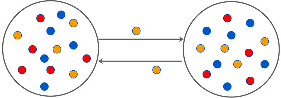	Fig. 1. (Color online) The schematic illustration of double-system with bidirectional time-varying migration. Red and yellow dots represent prey, blue represents predator, and yellow dots can migrate bidirectionally between the two subsystems.

According to the stochastic simulation schemes, one may write down the following set of dynamic equations at a mean-field level:
where x_i and y_i represent the densities of the prey without and with migration, respectively. z_i represents the density of predator, the subscript i (here i = 1, 2) is used to distinguish different subsystems. The parameters r_x (r_y), K_i, ε, and d are the birth rates of prey x(y), the maximum environmental carrying capacity of the subsystem i, the conversion rate of digested prey per unit time by predator and the mortality rate of the predator, respectively. is the logistic growth, representing the increase of the prey population in the absence of predator. In this model the per capita birth rate of x_i is , it is dependent on x_i + y_i. Namely, species x and y in the i-th subsystem are jointly restricted by the K_i, and the two species have competitive relations. F(x_i) and F(y_i) are the functional responses, denoting the amount of the prey killed by predator per unit time. Here, we employ Hollingʼs prey-dependent Type III functional response, i.e. n = 2. The same is true for . is a migration function of the prey y in the i-th subsystem at time t, which can be defined as follows
where, ω_ij indicates the migration rate of prey y from a subsystem i with high population density to another one j with low density. σ₁ is a rate representing the influence of the environment on the migratory process, for example, the channel effects among subsystems.

As we all know, the reasons of species migration in ecosystems are complex and there are many influencing factors,^[24] such as intra-population competition, reproductive migration, weather and environmental change, and even human influence, etc. Here, we assume that the prey migration is a time-dependent function related to the population density under the following consider.^[25] The increasement of the predator results in the prey decrease, which causes the predator decrease in turn; while the decreasement of the predator leads to the prey increase, and then render the predator increase. This phenomenon is similar to the memristor effect. Inspired by this, we build a time-varying migration function associated with population density by using the cubic flux-controlled memristor model as follows,^[26–27] which has been successfully applied to the biological neural networks:^[28–29]
where, ϕ_ij is the in-built variable of the memristor model, and α, β are the in-built parameters of the model, σ₂ is a tunable parameter that characterizes the competition within the migratory population.

In what follows, a fixed time step is set as 0.001. Other parameters r_x = 0.55, r_y = 0.71, h = 1.48, λ = 0.68, d = 0.485, α = β = 0.02, and the fourth-order Runge-Kutta method is employed to solve Eqs. (1)–(3).

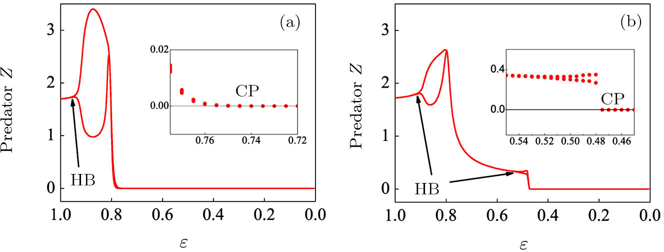
To begin, we select the conversion rate ε of digested prey per unit time by predator as the controll parameter to investigate the bifurcation behavior of the predator, and the range of ε belongs to (0, 1.0). The initial state of the system is randomly set to (x_i, y_i, , 0.9 + 0.2 × i, 1.6 + 0.3 × i). The numerical simulation result of Fig. 2 demonstrates the Hopf bifurcation diagram represented by the upper and lower values of predator Z dependent on parameter ε. For no migration, we set K = 10 and plot the predator population dynamics as a function of ε in Fig. 2(a). It is found that, with ε decreases from 1.0 to 0 the system undergoes a stable state to a Hopf bifurcation (HB), an unstable state of limit cycle, and a sharply decline, then means that the predator occurs extinction, i.e. Z = 0. In order to further study this phenomenon of population extinction, we stipulate that when the population density is lower than 10⁻⁵, it is considered that the population is extinct. As can be seen from Fig. 2(a), the predator enters the extinction state at a critical point (CP) ε_c = 0.740. The insets show a zoom of the closer region near CP. Next, we consider that the prey y migrates bidirectionally between two different subsystems (one with K₁ = 10 and another with K₂ = 5). We fix the parameters σ₁ = 0.8 and σ₂ = 0.5, and plot the bifurcation diagram in Fig. 2(b). One can observe that, as ε decreases from 1.0, the predator exhibits two-stage stable states ( (0.935, 1) and (0.540, 0.800)), and two-stage limit cycles ( (0.800, 0.935) and (0.480, 0.540)). Notice that the second Hopf bifurcation transition in the Fig. 2(b) becomes discontinuous when a migration is introduced compared to Fig. 2(a). However, unfortunately, we still do not know the underlying mechanism of this first-order like transition, since it is difficult to proceed to do linear stability analysis on the non-autonomous equation with a non-smooth time-varying migration. Anyway, the occurrence of this discontinuous transition means that the predator will suddenly become extinct at some specific parameter. Therefore, the physical significance of such a transition surely deserves further investigations. When , the predator becomes extinct. The insets of Fig. 2(b) also zoom the closer region of the CP. Obviously, the time-varying migration of the prey leads to the predator behaving richer dynamics than that without migration, including a significant decreasement of for the predator extinction, two HB points and two limit cycles. This phenomenon indicates that the migration would be very beneficial to preserve the species diversity of ecosystems.

Fig. 2.

	Figure Option ViewDownloadNew Window
	Fig. 2. The bifurcation diagram of the predator with parameter ε in the three-species PP system. (a) The single system without migration, K = 10. (b) The double-system with migration, K1 = 10, K2 = 5, σ1 = 0.8, and σ2 = 0.5. The insets shows a zoom of the closer region near the critical point (CP).

Figure 3 shows four typical phase portraits of prey and predator at different values of ε. When ε = 0.380, the system is in a stable state (7.148, 2.852, 0) as shown in Fig. 3(a), demonstrating the predator extinction. While ε = 0.490 and ε = 0.840, the system is in the unstable periodic state, limit cycles as shown in Figs. 3(b) and 3(c). When ε increases and arrives at 0.940, the system would be in a stable state (0.408, 1.393, 1.765), which suggests that three species coexist.

Fig. 3.

	Figure Option ViewDownloadNew Window
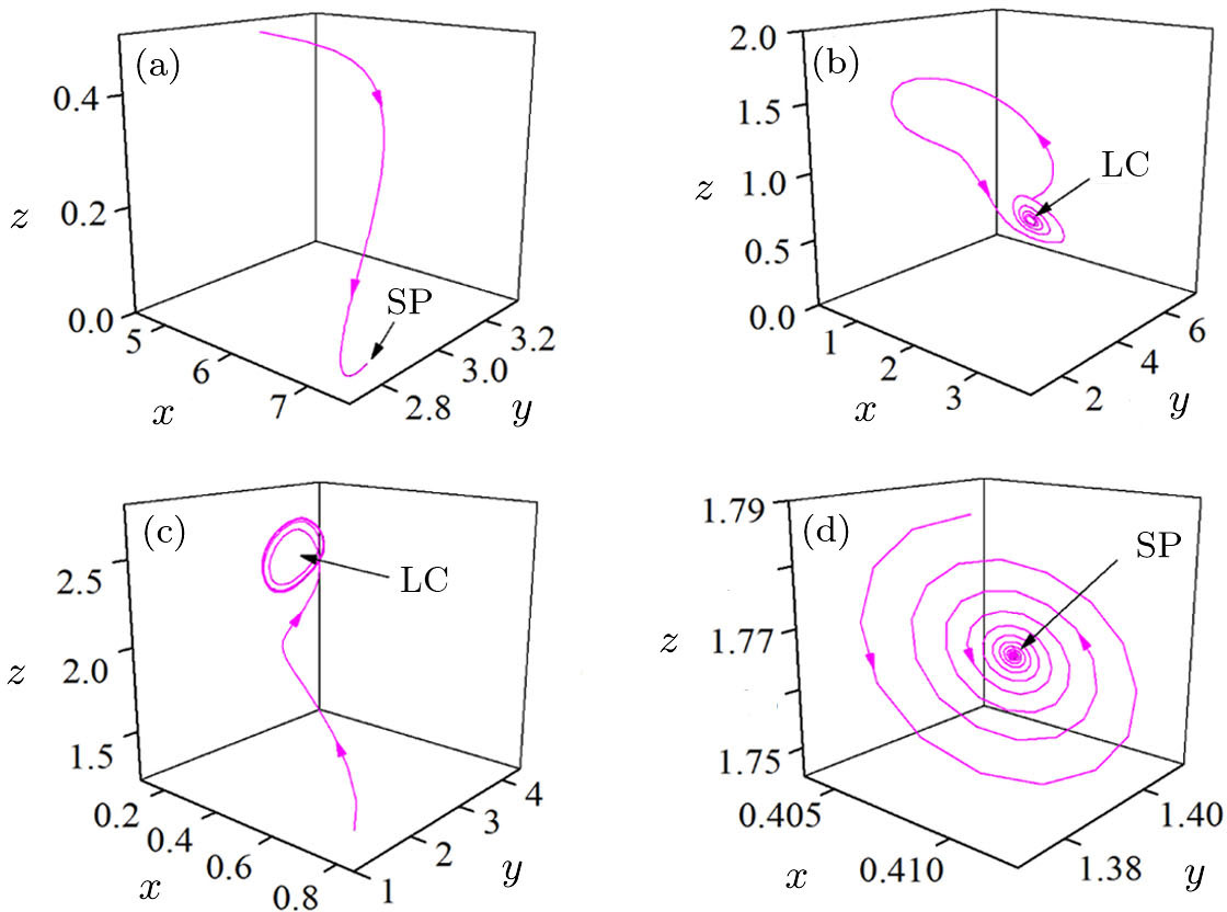
	Fig. 3. Four typical phase portraits of the double-system for ε = 0.38 (a), ε = 0.49 (b), ε = 0.84 (c), and ε = 0.94 (d).

To further investigate the influence of the migration parameters σ₁ and σ₂ on the critical point of predator extinction, we fix the step size of the migration parameters to be 0.001 to change between (0, 1) and stipulate that extinction occurs when the population density is less than 10⁻⁵. Firstly, we fix σ₂ = 0.5, and plot the ε_c as a function of σ₁, as shown in Fig. 4(a). It is found that as σ₁ increases, ε_c decreases monotonously, suggesting that the smaller influence of the environment impacts on the migration, the more favor of the predator coexists with the prey. While we fix σ₁ = 0.8, and one can find that ε_c increases monotonously with σ₂, as shown in Fig. 4(b). This indicates that the competition in the migratory process is not of benefit to the predator survival, since the predator needs more conversion rate of digested prey to avoid its extinction. Moreover, we made a Boltzmann fitting (red curve) in Fig. 4, which can show the change trend of ε_c depending on the migration parameters more intuitively. Figure 5 demonstrates the phase diagram of the predator extinction critical point in (σ₁, σ₂) plane. As can be seen from Fig. 5, when σ₁ (or σ₂) is in the fixed transfer function, the critical bifurcation parameter ε_c of predator extinction will increase (or decrease) with σ₂ (or σ₁) increases. Note that however, when the value of σ₁ is small, the change of σ₂ has little influence on the critical bifurcation parameter ε_c.

Fig. 4.

	Figure Option ViewDownloadNew Window
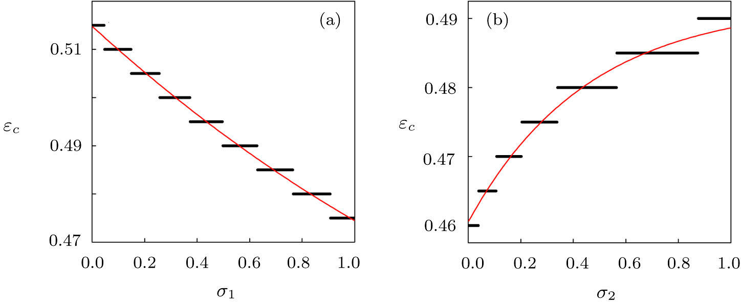	Fig. 4. (Color online) The critical parameter εc as a function of σ1 for σ2 = 0.5 (a) and as a function of σ2 for σ1 = 0.8 (b). Other parameters in the two-system model with migration are fixed as K1 = 10, K2 = 5, rx = 0.55, ry = 0.71, h = 1.48, λ = 0.68, d = 0.485, and α = β = 0.02.

Fig. 5.

	Figure Option ViewDownloadNew Window
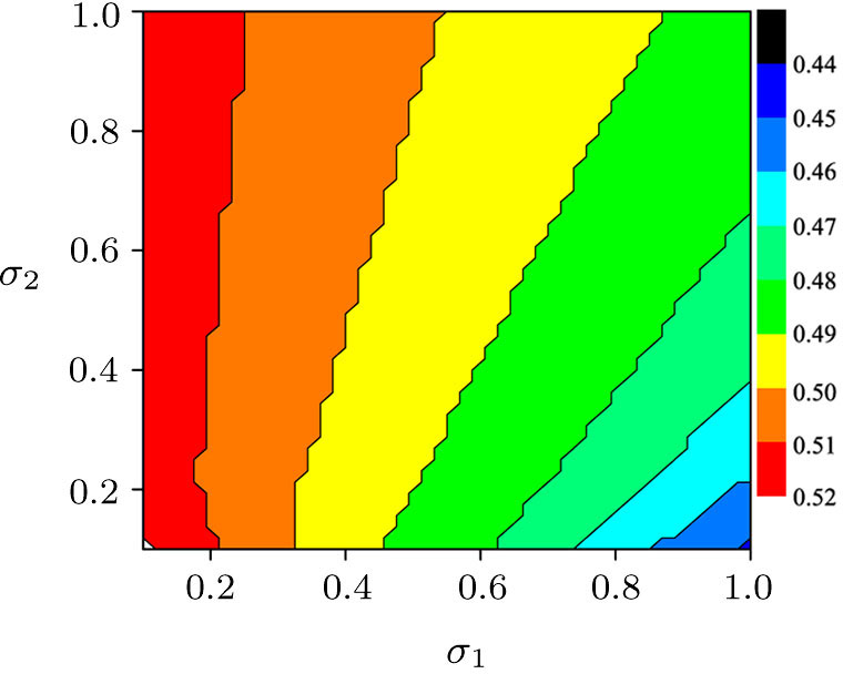
	Fig. 5. (Color online) The critical value of bifurcation parameter for predator extinction in two parameters phase diagram of σ1–σ2. Other parameters in the two-system model with migration are the same as those in Fig. 4.

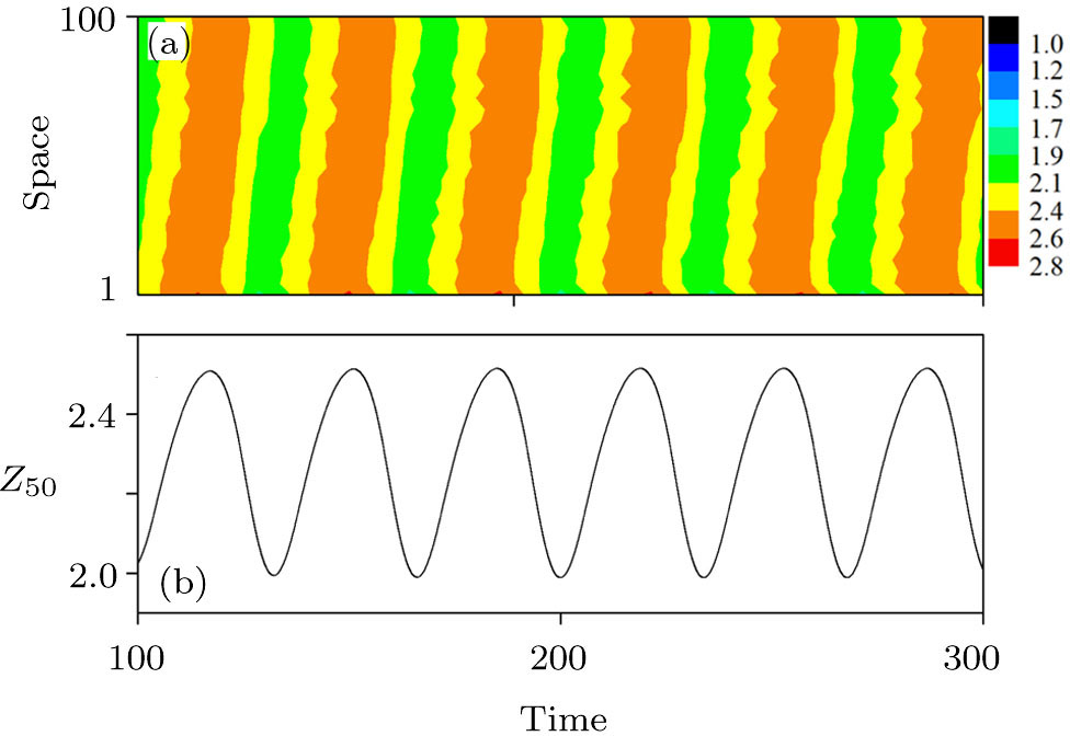
In addition, to check whether the population density evolves into a periodic solution when the pattern is formed, and also to further confirm that our proposed PP model with time-varying migration has the reliability of simulating real ecosystems, we allocate an array of subsystems with different maximum environmental carrying capacity and with , which ensures that any neighboring subsystem are not identical. Furthermore, a small Gaussian noise was added into K_i for all subsystems. We investigate the spatiotemporal dynamics of one-dimensional networked ecosystem consisting of 100 PP subsystems. Figure 6(a) shows that the one-dimensional multiple PP system with migration evolves into a fixed spatial pattern after a period of time, which is consistent with the phenomenon in the previous reports. Also, the time series z₅₀ of predator in the 50-th subsystem is plotted in Fig. 6(b) and one can observe that the system stabilizes into a periodic oscillation state ranging from 100 s to 300 s. The simulation results shown in Fig. 6 further confirm that the PP system model with time-varying migration function has the reliability to simulate real ecosystems.

Fig. 6.

	Figure Option ViewDownloadNew Window
	Fig. 6. (Color online) (a) Spatiotemporal pattern of the predator in one-dimensional space for multiple PP model with time-varying migration. (b) Time series of the predator in the 50th subsystem. The maximum environmental carrying capacity and with , other parameters ε = 0.82 and σ1 = σ2 = 0.5.

In summary, we have studied the effects of migration on the dynamics of three species PP system, which consists of one predator and two prey live in more than one subsystems. For simplicity, however, only one prey is considered to migrate among subsystems. To better characterize the feature of migration, we employ a cubic flux-controlled memristor model to construct a time-varying migration rate associated with the densities of subpopulation. By comparing the dynamic behaviors of PP system with and without migration, it is found that the three species PP system with migration exhibits rich dynamics, such as two Hopf bifurcations, two limit cycles, and a critical extinction point of the predator. Particularly, the migration of prey leads to the significant decrease of the critical value for the predator extinction, suggesting that the migration of prey is in favor of the survival of predator. In other words, if we intend to enhance the species diversity of an ecosystem, the prey should be driven to migrate between subsystems. Furthermore, we investigate the spatiotemporal dynamics of one-dimensional multiple PP system, and find that the system evolves into a stable evolution pattern after a period of time. Our results may provide valuable ideas for further study and preserving biological diversity in ecosystems.