


Vertical Sediment Concentration Distribution in High-Concentrated Flows: An Analytical Solution Using Homotopy Analysis Method
Cite this Article
Kumbhakar Manotosh, Saha Jitraj, Ghoshal Koeli, Kumar Jitendra, Singh Vijay P.. Vertical Sediment Concentration Distribution in High-Concentrated Flows: An Analytical Solution Using Homotopy Analysis Method. Communications in Theoretical Physics, 2018, 70(3): 367 
Permissions
Vertical Sediment Concentration Distribution in High-Concentrated Flows: An Analytical Solution Using Homotopy Analysis Method
† Corresponding author. E-mail:
Abstract
Abstract
Transport of suspended sediment in open channel flow has an enormous impact on real life situations, viz. control and management of reservoir sedimentation, geomorphic evolution such as dunes, rivers, and coastlines etc. Transport entails advection and diffusion. Turbulent diffusion is governed by the concept of Fick’s law, which is based on the molecular diffusion theory, and the equation that represents the distribution of sediment concentration is the advection-diffusion equation. The study uses the existing governing equation which considers different phases for solid and fluid, and then couples the two phases. To deal with high-concentrated flow, sediment and turbulent diffusion coefficients are taken to be different from each other. The effect of hindered settling on sediment particles is incorporated in the governing equation, which makes the equation highly non-linear. This study derives an explicit closed-form analytical solution to the generalized one-dimensional diffusion equation representing the vertical sediment concentration distribution with an arbitrary turbulent diffusion coefficient profile. The solution is obtained by Homotopy Analysis Method, which does not rely on the small parameters present in the equation. Finally, the solution is validated by comparing it with the implicit solution and the numerical solution. A relevant set of laboratory data is selected to check the applicability of the model, and a close agreement shows the potential of the model in the context of application to high-concentrated sediment-laden open channel flow.
1 Introduction
Transport of sediment in fluvial processes has been a long standing topic of research.[1–11] It plays a significant role in the control and management of reservoir sedimentation, geomorphic evolution such as dunes, river, and coastlines, etc. that have immense importance in our day to day life. Better understanding of sediment transport mechanism in natural watercourses needs knowledge of open channel flow. Sediment transport in open channel flow occurs mainly in two different modes, namely, bed-load and suspended load.[12] The part of the load that travels close to the bed is bed-load, while the other part travels in suspension as suspended load. In the study of suspended load, the spatial distribution of sediment concentration is of primary interest as it helps determine the discharge of suspended particles in watercourses, bed-load transport rate, and so on. The present study focuses on the vertical distribution of suspended sediment concentration in open channel turbulent flow.
The governing equation for sediment concentration distribution, termed as advection-diffusion equation (ADE), has the origin in Fick’s law of diffusion. Rouse[7] was the pioneer in this field to provide an analytical expression for vertical concentration profile by balancing the upward diffusion and the downward settling of sediment, and the solution provided by him is widely known as the Rouse equation. However, it has a major drawback that it cannot predict the sediment concentration values well near the channel bed or near the water surface, which might be due to the inclusion of Prandtl-von Kármán velocity profile that does not model velocities well in sediment-laden flows.[13] Following the work of Rouse,[7] different modifications have been done by researchers to overcome those drawbacks by incorporating several turbulent mechanisms.[6,9,11,14–15] On the other hand, Hunt[3] analyzed the dynamics of particle suspension by treating the fluid phase and the solid phase separately, and then coupled the phases by decomposing the vertical velocity of the particle into the vertical flow velocity and the particle settling velocity in a quiescent fluid. The Hunt equation has more practical importance, as unlike the Rouse equation, it can be applied to a region where the volume occupied by the particles is appreciable. For simplicity, Hunt[3] assumed the turbulent diffusion coefficient to be the same as sediment diffusion coefficient, which is a poor approximation valid only in the case of small particles as mentioned in his work. Later on, different experimental investigations revealed the non-equality of these coefficients for different flow conditions,[16–18] and different models on these coefficients are reported in literature.[9,19]
Numerous studies have been undertaken to investigate the vertical distribution of sediment concentration starting from the Hunt equation. But most of the researchers took the turbulent and sediment diffusion coefficients to be equal limiting the application of their studies. Very few researchers[6,20–21] considered the two coefficients to be different, and solved the equation numerically as the traditional analytical techniques did not succeed due to the non-linearity of the diffusion equation. To deal with the non-linear ODE-PDEs, classical perturbation[22] and asymptotic techniques[23–24] are widely applied to obtain analytic approximations of nonlinear problems in science and engineering. Unfortunately, perturbation and asymptotic techniques are too strongly dependent upon small/large physical parameters present in the governing equation, and thus are often valid only for weakly nonlinear problems.
The present study aims to derive an explicit analytical solution of the generalized diffusion equation with arbitrary turbulent diffusion coefficient, by means of a novel unified method, known as Homotopy Analysis Method (HAM). Liao[25] developed HAM to solve non-linear differential equations, which employs the concept of homotopy from topology to generate a convergent series solution for nonlinear systems. It has been proved[26] that the method is a unified one, which logically contains Lyapunov’s small artificial parameter method,[27] Adomian decomposition method,[28] Homotopy perturbation method (HPM),[29] the δ-expansion method,[30] and the Euler transform[31] as special cases. In summary, HAM distinguishes itself from various other analytical methods in three respects: (i) it does not directly rely on small physical parameters present in the governing equation; (ii) it assures the convergence of a non-linear differential equation; and (iii) it has flexibility regarding the choice of base functions and the auxiliary linear operator of the homotopy. Since its inception, HAM has successfully been applied to different fields of science and engineering.[32–44] The derived analytical solution obtained via HAM in the present study is validated with the implicit solution and with the 4th order Runge-Kutta (RK) method. The model is also compared with relevant experimental data on vertical sediment concentration of high-concentrated flow.
2 Mathematical Model
A sediment-laden flow of depth h in a wide open channel, in which the time-averaged suspended sediment concentration decreases monotonically from a maximum value Ca at the reference level y = a to zero at the water surface, is presented in Fig.
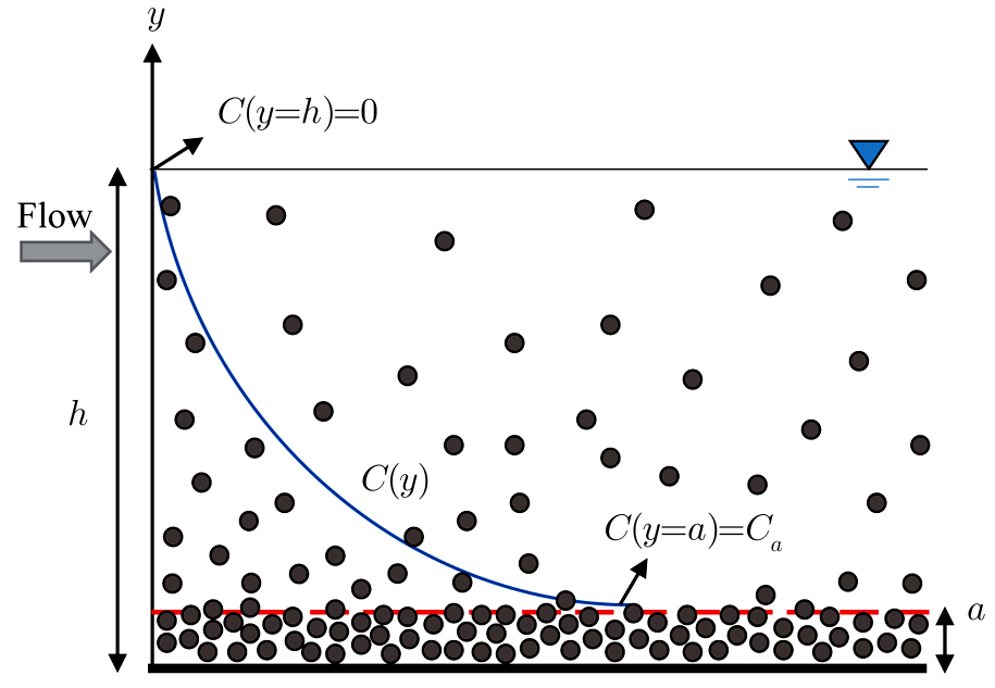 | Fig. 1 Schematic diagram of sediment concentration distribution along a vertical in open channel turbulent flow over a sediment bed; within the reference level y ≤ a, sediments move as bed load, and above that as suspended load. |
2.1 Governing Equation2 ) is inserted in the governing equation (1 ).4 ) is a first-order highly non-linear ordinary differential equation, which represents vertical distribution of suspended sediment concentration. The solution methodology for solving Eq. (4 ) is described in what follows.
In the case of steady-uniform flow where sediment concentration varies only in the vertical direction, the generalized governing equation can be written as:[3]

Experimental observations revealed that in the case of flow with suspended sediment particles, the flow around the neighboring settling particles exhibits a larger drag as compared to the clear water flow, known as hindered settling effect. This effect reduces the settling velocity in a sediment-laden flow from that in a clear fluid. The widely used expression for ωs was proposed by Richardson and Zaki,[46] which reads as:

The expression for εs(y) or εt(y) should be available to determine the profile of vertical concentration distribution, as can be noticed from Eq. (
Before proceeding further, we rearrange Eq. (

2.2 Implicit Solution Obtained for Eq. (4 ) without and with Hindered Settling Effect
5 ), we obtain
4 ) can be rearranged as:

8 ) is quite accurate due to the smallness of C in the region [a, h]. Using the approximation Eq. (8 ) in Eq. (7 ), and then integrating using the boundary condition, one can obtain the implicit solution in the following form:
6 ) and (9 ) represent implicit solutions for the vertical sediment concentration distribution without and with the effect of hindered settling, respectively. The right hand side of Eqs. (6 ) and (9 ) can easily be integrated with the substitution of linear and parabolic profiles for K(z) mentioned previously.
Without the effect of hindered settling, i.e., nH = 0, Eq. (


However, Eqs. (
2.3 Solution Obtained by HAM


13 ) converges at q = 1. Then, at q = 1, the series becomes
14 ) provides the relationship between the initial approximation C0(z) and the exact solution C(z). However, the higher order approximations Cm(z) for m ≥ 1 are still unknown to us. Liao[25] showed that the higher order terms can be obtained by differentiating the zeroth order deformation Eq. (11 ) (with 
18 ), in accordance with Liao’s rule of solution expression, a single-term linear operator is chosen in order for simplicity of the subsequent derivations:

17 ), the first few terms are calculated as follows (“′” represents first-order derivative with respect to the independent variable z):
18 ) as follows:
19 ), and using the boundary condition 
26 ) that one can obtain the iteration as per wish once the initial approximation C0(z) is known. For subsequent derivations, the initial approximation 
We suggest this unified method, HAM, not only for solving the equation modeled in this study but for any strong non-linear problem arising in the field of hydraulics, especially sediment transport phenomenon; therefore, for the sake of completeness, here we briefly present the methodology (as proposed by Liao[26]) associated with it in a convenient way. For that purpose, let us consider the original non-linear Eq. (


The term (1 − C)nH + 1 presents in the governing equation involves a non-integer exponent, which makes the equation highly non-linear and may take longer computational time when applying HAM. Thus, before proceeding further, we use some accurate approximation for that term similar to Eq. (


3 Results and Discussion
In this section, we validate the HAM-based solution given by Eq. (
3.1 Selected Expressions for the Parameters
29 ). The Rouse number A : = ω0/βκu* is computed using the expressions for ω0 and β given by Eqs. (28 ) and (29 ), respectively. The parameter κ is a universal constant having the value 0.41. Calculation of the reference level 


It is to be noted that in order to apply the derived analytical model (Eq. (

On the other hand, investigations on the determination of expression for β have been limited since the start.[9,19] Recently, Pal and Ghoshal[19] studied the nature of β by analyzing a large number of data sets of different researchers, and established two relations of β for dilute and non-dilute flows. Their study claims that β values do not only depend upon normalized settling velocity, but also on reference level and reference concentration. They developed the following expressions:
3.2 Validation of the HAM-Based Solution
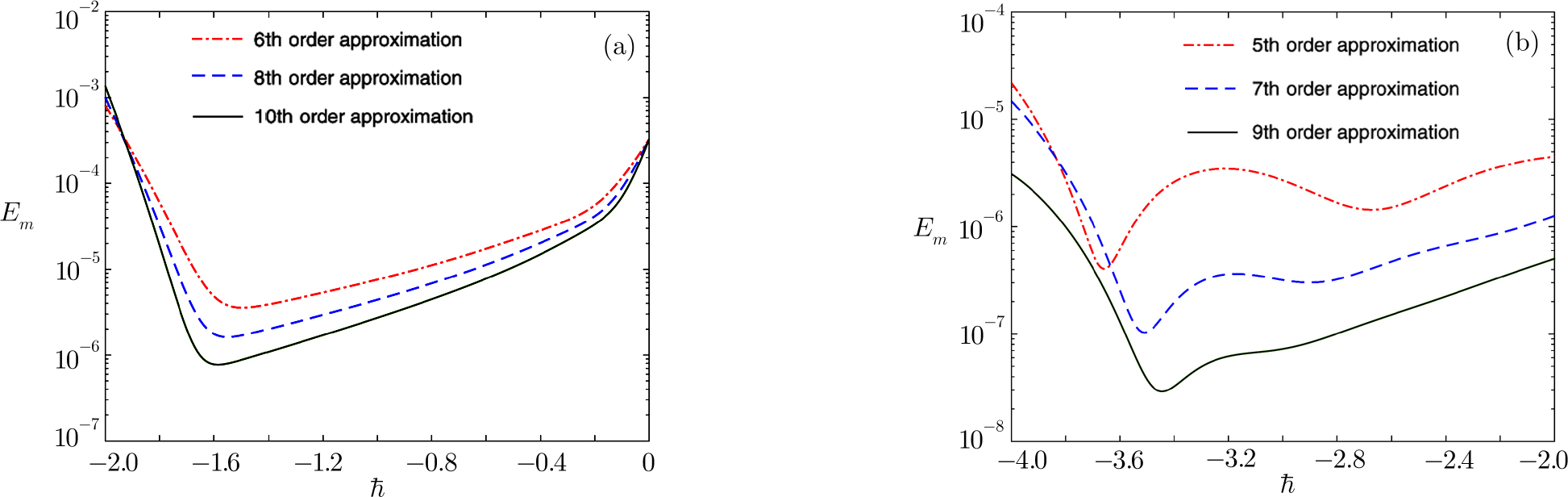
It can be observed that the HAM-based series solution given by Eq. (
 | Fig. 2 Average residual error Em versus the auxiliary parameter ℏ taking A = 1, α = 0.5, nH = 4,   |
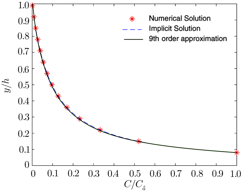
Now, we validate the obtained HAM-based solution by comparing it with implicit solution given in Eqs. (
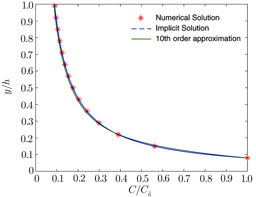
 | Fig. 3 Validation of the HAM-based solution (for ℏ = −1.585) with numerical solution (4th order RK-method) and implicit solution considering linear profile for K(z). A = 1, α = 0.50, nH = 4, a/h = 0.08, Ca/h = 0.02, K(z) = z. |
 | Fig. 4 Validation of the HAM-based solution (for ℏ = −3.445) with numerical solution (4th order RK-method) and implicit solution considering parabolic profile for K(z). A = 1, α = 0.50, nH = 4, a/h = 0.08, Ca/h = 0.02, K(z) = z(1 − z). |
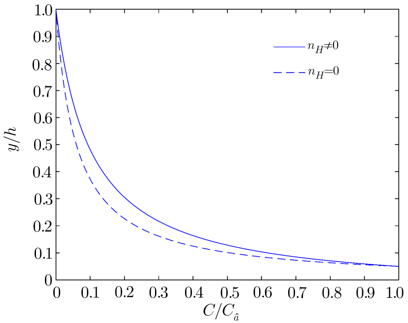
3.3 Variation of Concentration Profile with nH and A
The effect of hindered settling on vertical sediment concentration profile is shown in Fig.
 | Fig. 5 Influence of hindered settling through nH on the vertical concentration profile. A = 1, α = 0.25, a/h = 0.05, Ca/h = 0.10. |
Figure
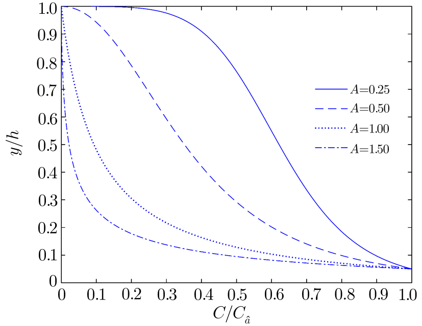
In Fig.
 | Fig. 6 Vertical concentration profiles for different values of the Rouse number A. a/h = 0.05, Ca/h = 0.10, nH = 4, α = 0.25. |
3.4 Further Modification to the Solution and Application to Laboratory Data
20 ). Therefore, the final solution was obtained, considering parabolic profile for K(z), as follows:

24 ).
According to Liao’s rule of solution expression, one can choose the initial approximation, auxiliary linear operator, and auxiliary function with great freedom. In the previous section, we obtained the HAM-based series solution by choosing these functions. However, the solution obtained was seen to be close to the numerical solution for terms considering up to 9th order or so. Here, we further refined our choices of these functions, in accordance with the rule of solution expression of HAM, to search for a reliable 3rd–4th order analytical solution to the problem. To that end, {((1 − z)/z)n; n ≥ 0} was chosen as the set of base functions to represent the solution C(z) for the problem. Accordingly, the auxiliary linear operator 
The present study considered the most generalized governing equation by taking into account the physics of sediment-laden flow through the incorporation of hindered settling effect, arbitrary K(z) profile, and the non-identity of the ratio of sediment diffusion coefficient to turbulent diffusion coefficient. Specifically, the equation modeled here is applicable for high-concentrated flows. To check the applicability of the model, a relevant set of laboratory data was chosen for verification. Experimental data of Einstein and Chien[54] was selected for verification as it is the most cited data for high-concentrated flows. They carried out their experiments in a recirculating flume of 12.2 m length and 30.7 cm width for three different particle sizes, namely, 0.274 mm, 940 mm, and 1.3 mm. The sediment concentration distribution near the channel bed is always a difficult task to measure, as it is under the influence of both sediment concentration and the channel bed, and hence, is of great importance. Einstein and Chien[54] measured concentration values very close to the channel bed, and reported 16 different measurement runs, named Run S1 to S16. We selected three test cases having three different particle diameters: S1 (1.3 mm), S6 (0.940 mm), and S12 (0.274 mm) for validation.
Figures
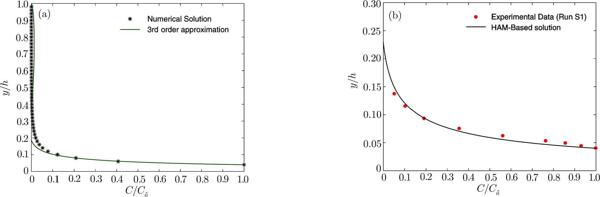 | Fig. 7 Validation of the HAM-Based Solution (Eq. ( |
| Table 1 Summary of the selected experimental data from Einstein and Chien[17] for high-concentrated sediment-laden flow. . |
It is observed that only the 3rd order approximate solution obtained by HAM given in Eq. (
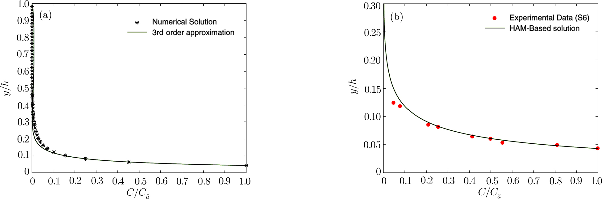 | Fig. 8 Validation of the HAM-Based Solution (Eq. ( |
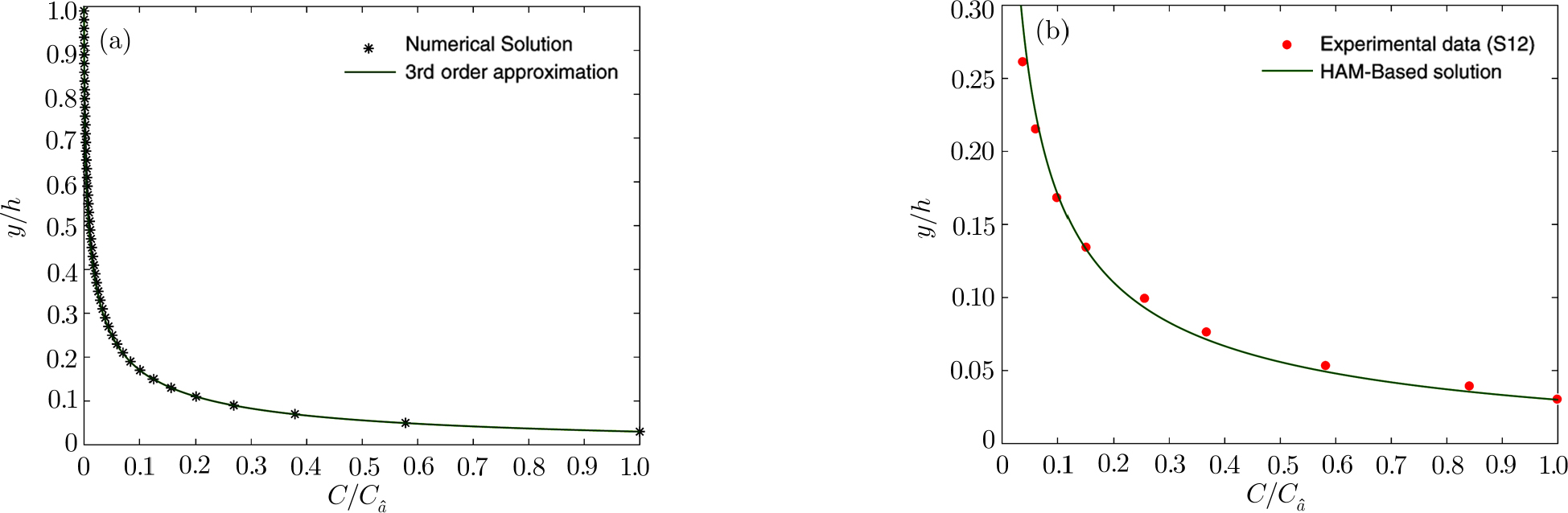 | Fig. 9 Validation of the HAM-Based Solution (Eq. ( |
4 Conclusions
The following conclusions can be drawn from this study:
The study derives an explicit analytical solution to the most generalized governing equation for suspended sediment transport in open channels using a powerful mathematical tool, known as Homotopy Analysis Method (HAM). The method derives the solution for an arbitrary turbulent diffusion coefficient profile. Unlike the classical perturbation techniques, HAM does not rely on the presence of small/large parameters in the governing equation. Besides, the method is a generalized one, which contains several other analytical methods such as ADM, HPM, classical perturbation method etc. as special cases, and it paves the way for monitoring the convergence of the series solution through an auxiliary parameter. In all, the method can be applied to the field of hydraulics where non-linear differential equations often arise. The governing equation for vertical sediment concentration distribution is formulated considering the different phases of fluid and solid, and then coupling both of the phases: a concept which was originally developed by Hunt, and the corresponding equation is widely known as the Hunt equation. To deal with high-concentration flow which is of great importance, sediment and turbulent diffusion coefficients are assumed to be different from each other. The effect of hindered settling on sediment particles is included in the model, and the concentration profile is analyzed due to this effect, which explains the real physics associated with high-concentrated flows. To assess the derived analytical solution, required parameters are computed from the recent studies of the corresponding parameters. An implicit solution to the governing equation is also obtained for validating the HAM-based solution. Furthermore, the implicit solution, HAM-based solution, and the numerical solution (the 4th order RK method) are compared for different test cases considering two different profiles for eddy viscosity, namely, linear and parabolic profile. At the end, the HAM-based solution is further achieved for different choices of the linear operator and the initial approximation to the solution. The derived solution is then seen to be close to the numerical one only for three terms of the series. Finally, to check the applicability of the derived model, a widely cited laboratory dataset on vertical concentration profile in high-concentrated flow is selected. A close agreement is found between the observed and computed values, which shows the potential of the model in the context of application to the high-concentrated free surface sediment-laden flows.
Reference
| [1] | |
| [2] | |
| [3] | |
| [4] | |
| [5] | |
| [6] | |
| [7] | |
| [8] | |
| [9] | |
| [10] | |
| [11] | |
| [12] | |
| [13] | |
| [14] | |
| [15] | |
| [16] | |
| [17] | |
| [18] | |
| [19] | |
| [20] | |
| [21] | |
| [22] | |
| [23] | |
| [24] | |
| [25] | |
| [26] | |
| [27] | |
| [28] | |
| [29] | |
| [30] | |
| [31] | |
| [32] | |
| [33] | |
| [34] | |
| [35] | |
| [36] | |
| [37] | |
| [38] | |
| [39] | |
| [40] | |
| [41] | |
| [42] | |
| [43] | |
| [44] | |
| [45] | |
| [46] | |
| [47] | |
| [48] | |
| [49] | |
| [50] | |
| [51] | |
| [52] | |
| [53] | |
| [54] | |
| [55] |