1 IntroductionSince the concept of  -symmetry was raised by Bender and co-workers,[1–2] in the past decade there has been growing interest in the study of this area due to the fact that non-Hermitian
  -symmetric Hamiltonian extends the framework of quantum mechanics into the complex domain. Although in recent years much work has been done on the theoretical side of this issue,[3–12] up till this day, there has not been genuine experimental realization of
  -symmetric quantum system yet, because the
  -symmetry requires V(x) = V*(−x) for one-dimensional Hamiltonian, which demands existence of complex potential for the system, something hard to realize despite the theoretical proposal.
Fortunately, the study of  -symmetry found its cast in the field of optics, thanks to the isomorphism between Schrödinger equation and optical paraxial wave equation. For this reason, many endeavors have shown up in realizing
  -symmetric optical metamaterials in recent years. On one hand, artificial optical materials have already shown the advantages for achieving unusual electromagnetic properties compared to natural media, not to mention the fact that the
  -symmetry will certainly open up the gate to more intriguing properties, like double refraction and band merging,[13–14] power oscillations,[15–16] coherent perfect absorbers,[17–19] unidirectional invisibility,[14,20–21] and so on. However as a matter of fact, most of these works are carried out on solid-state optical systems, without much attempt to utilize atomic lattices. Considering that atomic optical lattices have their big advantages in real-time, all-optical tunable and reconfigurable features in control as compared to solid-state systems, it is of valuable importance to extend the study of
  -symmetry to this area. In recent years several works have come into sight[22–26] on this aspect.
For study of  -symmetry in optical field, when mapping the time-dependent Schrödinger equation to the paraxial wave propagation equation, the role of time variable t in Schrödinger equation is cast to the spatial variable of propagation direction (we use z in this work) in paraxial wave equation, and the
  -symmetry condition V(x) = V*(−x) is mapped to the complex refractive index symmetry n(x) = n*(−x) in transverse plane of propagation. Many works have been done under this scheme.[15–16,27–33]
On the other hand, the question has been asked about what if we implant the symmetric modulation of complex refractive index n to the longitudinal direction instead of transverse plane of optical wave propagation.[34] Inspired by this, we propose the scheme of realizing complex refractive index symmetry along the propagation direction of one-dimensional atomic optical lattices.
Surprisingly and most interestingly, in our study we find that under spatial sinusoidal detuning setting along propagation direction, 1D atomic lattices of any configuration could uniformly demonstrate pseudo- -antisymmetry, by which we mean n(z) = −n*(−z), where z denotes the propagation axis. When being cast back to quantum-mechanical side, this corresponds to V(x,t) = −V*(x,−t), the conjugate time-reversal antisymmetry of complex potential V(x,t) in Schrödinger equation.
The phenomenon of universal inducement of pseudo- -antisymmetry goes beyond our usual recognition that the optical features of atomic lattices are predominantly related to the energy level configuration of atoms, which together with particular setting of applied fields determine the optical response features of the lattice. Rather, it must originate from some fundamental physical features in the atomic optical lattice system, so that it could not see the difference between configuration details. And we find that the reason for this phenomenon is the quantum-mechanical nature described by master equation under weak probe field approximation.
The article is organized as follows. In Sec. 2 we define the concept of pseudo- -antisymmetry. In Sec. 3 we give the proof of universal inducement of pseudo-
 -antisymmetry under spatial sinusoidal detuning setting. In Sec. 4 we present an example of pseudo-
 -antisymmetry inducement on the family of zigzag-type configurations. And finally in Sec. 5 we conclude the article.
2 Pseudo- -antisymmetry
The effects of parity operator  and time-reversal operator
  on quantum-mechanical coordinate operator
  and momentum operator
  are
are
with

and

,

commute with each other. Since a

-reflected Hamiltonian is defined as
and the

-symmetry requires that

, for one-dimensional Hamiltonian
, the

-symmetry comes down to

This suggests a complex potential setting, which is not normally applicable in physical experimental environment. However the complex potential
V has found its cast in the complex refractive index
n in optics.
Optical lattice can be looked on as non-magnetic medium with no free charges or currents in it, then for electric field propagation we have the Helmholtz equation
where
z is the variable on propagation axis of 1D atomic lattices,

stands for any vector in transverse plane,
ω the angular frequency of the electromagnetic wave oscillation, and
c the speed of light in vacuum. In homogeneous media, Eq. (
3) reduces to a scalar equation.
In our one-dimensional optical lattice model, n could be designed as the periodic function of z, i.e. n(z + a) = n(z), where a is the spatial period of 1D optical lattice. Including the real background refractive index n0, we have n(z) = n0 + δn(z), with δn(z) = nR(z) + inI(z) being complex and |δn(z)| ≪ |n0|. The propagating electric field is given by E(x, z) = ϕ(x,z)eik0z, where ϕ (x,z) is the envelope function. Then under paraxial approximation, the scalar Helmholtz equation reduces to

where
k0 =
n0ω/
c,
is the effective potential. Notice however, that Eq. (
4) is not the analog of one-dimensional Schrödinger equation
because the genuine analog requires that time variable
t in Eq. (
5) be cast to longitudinal variable
z in paraxial wave equation, and spatial variable
x in Eq. (
5) be cast to transverse variable
x, which is to say,
V in Eq. (
4) should be a function of
x, not a function of
z. This means the normal

-symmetry requires the complex refractive index to satisfy
δn(
x) =
δn*(−
x) in transverse plane, with no restriction set for
z direction for 1D optical lattices. Compared to this, what we realized in this paper is
δn(
z) = −
δn*(−
z) along the propagation direction of 1D atomic lattices. From the point of view of

-symmetry,
δn(
z) = −
δn*(−
z) corresponds to the condition

which is the conjugate time-reversal antisymmetry of complex potential
V(
x,
t), and we call it pseudo-

-antisymmetry. We expect the study on the optical side could eventually shed light on the quantum-mechanical side, for interest of investigating
V(
x,
t) = −
V*(
x,−
t).
One may ask why in casting back the pseudo- -antisymmetry to Schrödinger equation, both variables x and t are included in potential V, while in Eq. (2) only variable x is shown. This comes from the features of 1D atomic optical lattices, which cause the difference between paraxial wave equation and Schrödinger equation in spite of the isomorphism. Since the atomic lattices are constructed by forming dipole traps to trap the atoms, there is density distribution in transverse plane, which affects the complex refractive index n, so n is not only function of z, but also x. However along the z axis of atomic optical lattices, settlement on any value of x does not affect the pseudo-
 -antisymmetry, so we can express n as n(z).
3 Universal Pseudo- -antisymmetry on One-dimensional Atomic Lattices
For any atomic configuration, the density matrix equations of off-diagonal terms can be expressed in the general form of master equation
The Hamiltonian can be written as

, where

is the Hamiltonian of free atom, and

the interaction between atom and applied fields. Then since
, the master equation becomes

where
ωnm = (
En −
Em)/
ħ =
ωn −
ωm is the resonant transition frequency between energy level
n and
m of the atom.
On 1D atomic lattices, we are applying a weak field to probe the optical response. Compared to all the other strong coupling fields, this is a perturbation, therefore we can turn to the traditional perturbative calculation method in nonlinear optics to carry out our calculation.
First suppose all external fields are treated as perturbation, then from Eq. (7), we have the first and second order perturbed ρnm expressed as


where the perturbation

is defined as
, with
E(
t′) =
E(
ωf(nm)) e
−iωf(nm)t′ being the field coupling energy states |
n⟩ and |
m⟩ on the relevant dipole moment
dnm, and
ωf(nm) the frequency of the coupling field. Since we have

therefore

and we can derive from here

where
N is the atomic distribution function.
To get the second order perturbed density matrix term  , normally we should directly bring the result of
  into Eq. (9) for a second round calculation. But things get different here when using weak probe field approximation. Because the probe field is so small compared to the strong coupling fields, in the first round calculation of
  , we usually ignore the existance of the probe field. Then when calculating
  , we begin to include the effect of probe field. This is to say, the
  in Eq. (8) and Eq. (9) are different by an addition of probe field. And the optical response of the probe field is the difference between the original
  without throwing in probe field
and that after throwing in the probe field

where under the assumption that the probe field is coupled to energy level |
k⟩ and |
l⟩,

We then see the change of

by applying the weak probe field is
On the other hand, it is straightforward to get

since this is analogous to the expression in Eq. (
10), comparing with
following the same path we have
This is the expression of weak probe field susceptibility. Now we relate this to the spatial sinusoidal field detuning set. We get this idea from solving the zigzag-type configuration problems, which we will present as an example in the next section. We rewrite the above expression as
The part i(
ωkl −
ωf(kl)) in the denominator is by definition the term iΔ
d, where Δ
d is the frequency detuning of the probe field. So in a generalized way, we can say that the denominator can be expressed as the polynomial in the indeterminate iΔ
d in the form
knowing
γkl can be looked on as
γkl(iΔ
d)
0. On the other hand, for the numerator, both

and

are real numbers that can be expressed in form
which is a special case of Σ
j=0Aj(iΔ
d)
j. Therefore we can say the expression of Eq. (
14) is a special case of expression
where
N1 is the highest order of indeterminate iΔ
d in the numerator’s polynomial, and
N2 the highest order of iΔ
d in the denominator’s polynomial. If we can prove that the expression in Eq. (
15) can have the universal pseudo-

-antisymmetry, then it will also work on its special case, Eq. (
14).
Equation (15) can be rewritten as

where
C2m,
C2m+1 (
m = 0, 1, 2, . . . ) and
D2p (
p = 0,1,2, . . . ) are real coefficients from rearranged polynomials of
Aj (
j = 0, 1, . . .,
N1) and
Bl (
l = 0,1, . . .,
N2). Normally for 1D atomic lattices,
N =
N(
z) is the periodic Gaussian distribution function of the atom density, which can be expressed as

where
z0i is the
i-th lattice center,
a the length of the lattice unit (also the spatial period of the 1D optical lattice),
N0 the density of atoms at lattice center, and
σ the standard deviation of the Gaussian distribution. We can always choose an appropriate reference point
z0 (in this case, any
z0i) to make
N(
z) an even function about
z0. After that, it is straightforward to see that if we set the coupling field frequency detuning Δ
d to be a sine function of
z axis, i.e.,

where
A represents the real amplitude of the oscillation, then about the reference point
z0 along
z direction, Re

is an odd function and Im

is an even function, which indicates the realization of pseudo-

-antisymmetry
n(
z) = −
n*(−
z).
We have proved that under spatial sinusoidal detuning setting, a probe field susceptibility described by Eq. (15) will demonstrate pseudo- -antisymmtry. Since under the weak probe field approximation, the probe susceptibility of 1D atomic lattices of any configuration can always be expressed by Eq. (14), a special case of Eq. (15), we have arrived at the conclusion that the sinusoidal detuning setting can induce universal pseudo-
 -antisymmtry on 1D atomic optical lattices, regardless of energy level configuration.
In the next section we will present an example of universal pseudo- -antisymmtry inducement on the zigzag-type configuration family of 1D atomic lattices, where we first found the idea of sinusoidal detuning setting in our early study, and where we got our first inspiration on the general case proof shown above. Without this first inpiration we would not be able to get the general case proof shown in this section.
4 Universal Pseudo- -Antisymmetry on Zigzag-Type Configuration Family: An Example
4.1 Case Study: N Configuration(i) The Model
We first point out that the control of n is equivalent to modulating probe susceptibility χp. Since  , and from Sec. 2 we know that n = n0 + δn with n0 being the background refractive index, also for atomic optical lattices n0 = 1, so we have δn = χp/2.
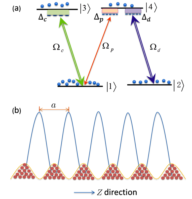
We design a system of one-dimensional optical lattice, composed of Gaussian-distributed bunches of cold 87Rb atoms, with each bunch seated at the bottom of a dipole trap along z direction, and atoms coherently driven into N-type configuration by three coherent laser fields applied to the system, at frequencies (amplitudes) ωp (Ep), ωc (Ec), and ωd (Ed), as shown in Figs. 1(a) and 1(b). The N-configuration consists of two ground levels |1⟩ and |2⟩ and two excited levels |3⟩ and |4⟩, and the weak probe field ωp interacts with the dipole-allowed transition |1⟩ ↔ |4⟩, while the two strong pump fields ωc and ωd act upon transitions |1⟩ ↔ |3⟩ and |2⟩ ↔ |4⟩, respectively. The corresponding frequency detunings are defined as Δp = ωp − ω41, Δc = ωc − ω31, Δd = ωd − ω42, and the Rabi frequencies Ωp = Ep · d14/ħ, Ωc = Ec · d13/ħ, and Ωd = Ed · d24/ħ, with ωij = ωi − ωj being resonant transition frequencies and dij the relevant dipole moments (i, j are labels of the energy levels).
With rotating-wave and electric-dipole approximations, the interaction Hamiltonian can be written as
We then get the density matrix equations:
where
,
,
,
,
,
; and Δ
12 = Δ
p − Δ
d, Δ
23 = Δ
c + Δ
d − Δ
p, Δ
34 = Δ
p − Δ
c.
We also assume Γ
31 = Γ
32 = Γ
41 = Γ
42 =
γ, and
γ12 ≪
γ, therefore
γ13 =
γ14 =
γ23 =
γ24 =
γ,
γ34 = 2
γ. Closure of this atomic system requires that

and
ρ11 +
ρ22 +
ρ33 +
ρ44 = 1.
(ii) A Special Case of Pseudo- -Antisymmetry on N Configuration
Using weak probe field approximation, we obtain the first-order steady-state solutions of Eqs. (19), and since we are interested in the probe field, we directly go for the expression of  . For simplicity, we set γ12 = 0 and look at the special case

then obtain
Here we have uniformly replaced all the Δ
c by Δ
d, while still writing down Ω
c and Ω
d separately. The reason of doing this will be explained later.
We can see that under the assumption that Ωc = Ωd are real numbers, both the numerator and the denominator of the formula can be expressed as polynomials in indeterminate iΔd, i.e.,
where
N1 is the highest order of term iΔ
d in numerator, and
N2 the highest order of iΔ
d in denominator.
Aj (
j = 0,1, . . .,
N1) and
Bl (
l = 0,1, . . .,
N2) are real coefficients determined by Eq. (
21). The expression of Eq. (
22) goes back to the form of Eq. (
17), using
χp =
N|
d14|
2ρ41/2ϵ
0ħΩ
p and setting
N(
z) to be the periodic Gaussian distribution function described by Eq. (
17), we realize pseudo-

-antisymmetry
n(
z) = −
n*(−
z) for 1D optical lattice on
N-configuration.
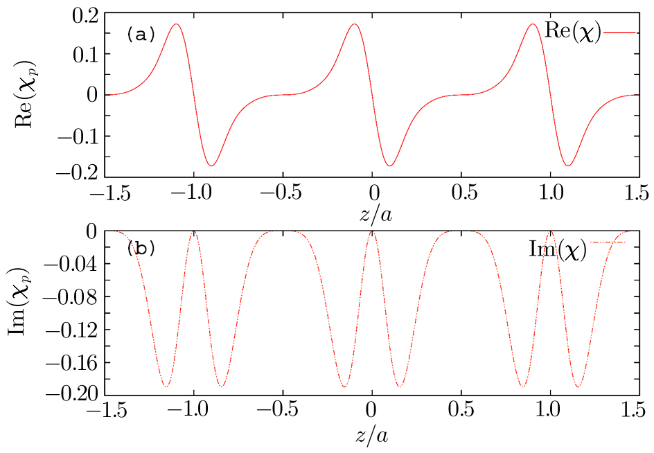
In Figs. 2(a) and 2(b) we plot the real and imaginary parts of probe susceptibility χp as function of z. The parameters used here are Ωc = Ωd = 5 MHz, Ωp = 0.06 MHz, Γ31 = Γ32 = Γ41 = Γ42 = 3 MHz. For the frequency detuning function Δd = A sin[2π(z − z0)/a], we choose z0 = 0 and set A = 1 MHz.
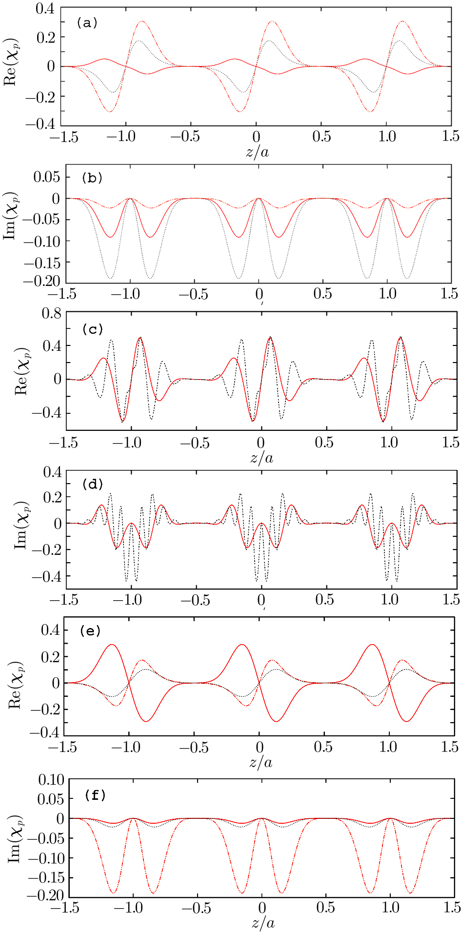
(iii) Pseudo- -Antisymmetry on N Configuration under Modified Parameters
Setting Δc = Δd in Eq. (20) ensures the expression of ρ14 in Eq. (21) to be a function of indeterminate iΔd, however, loosening this condition to
where
A1 ≠
A2 are both real amplitudes, we still get the pseudo-

-antisymmetry, as shown in Figs.
3(a) and
3(b).
We can also modify the periods instead of amplitudes of the sine functions by setting
where
m and
n are different integers, and we get the modulated periodical spatial distribution of
χp, which still satisfies the pseudo-

-antisymmetry as shown in Figs.
3(c) and
3(d).
For the condition Ωc = Ωd in Eq. (20), we change them to different values and still get the pseudo- -antisymmetry. The results are shown in Figs. 3(e) and 3(f).
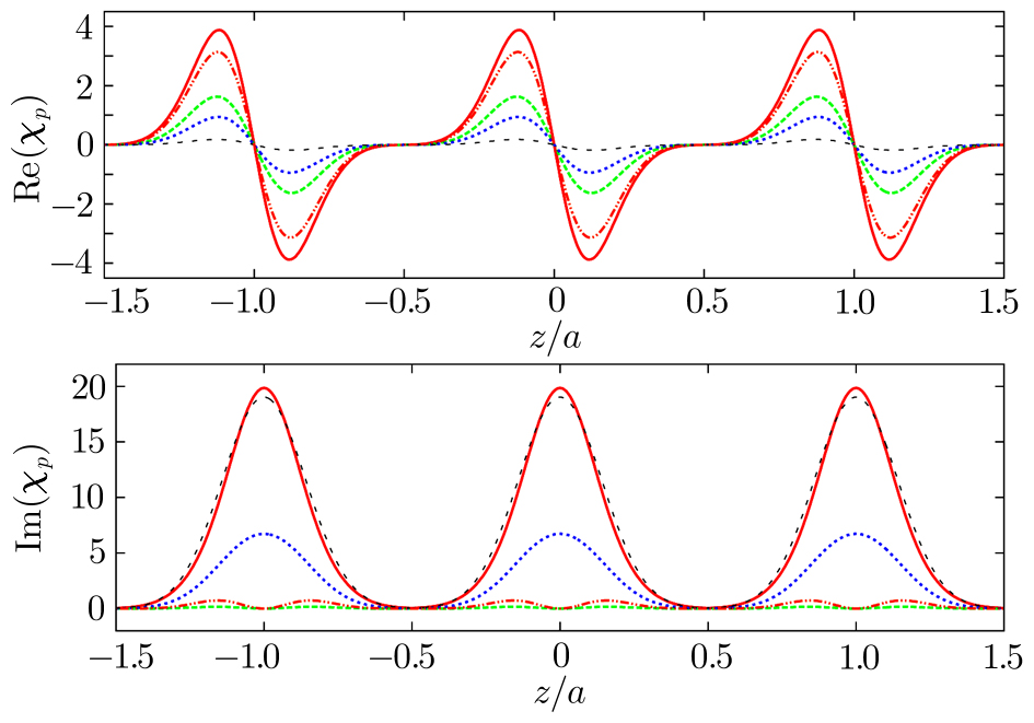
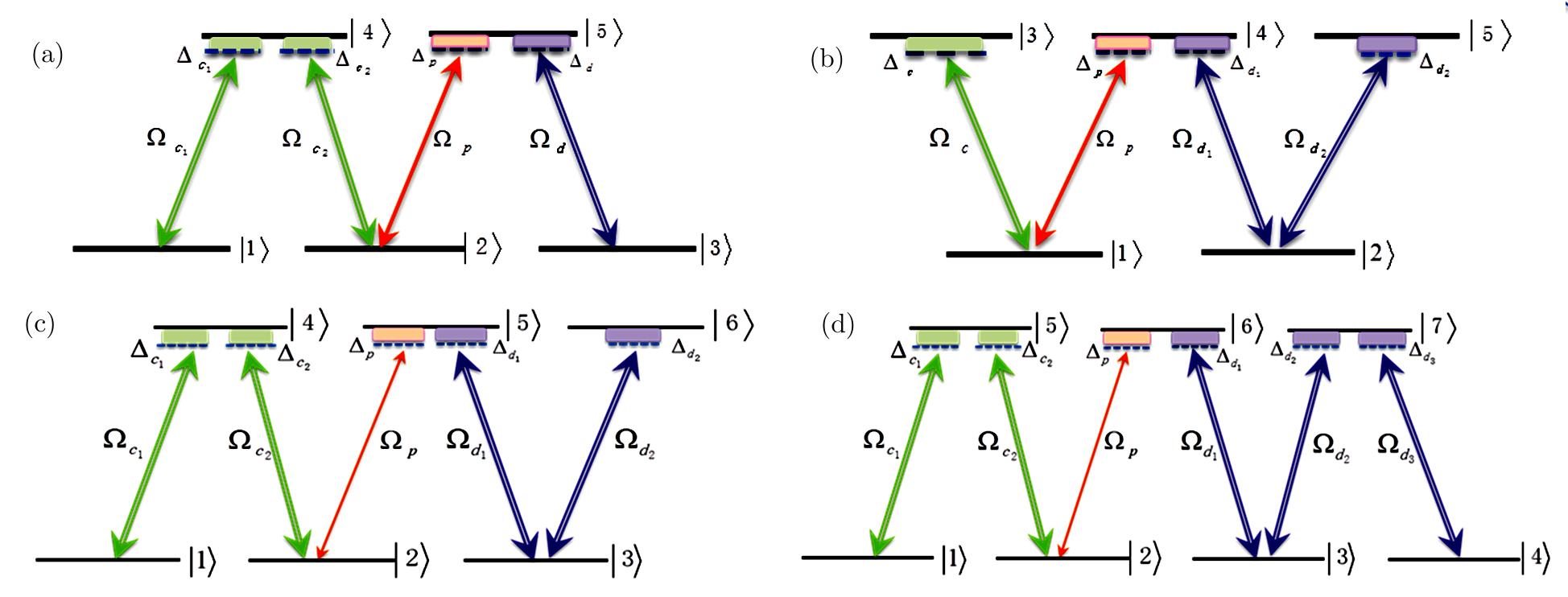
4.2 Numerical Study on Different Zigzag ConfigurationsWe now look at the different zigzag-type atom configurations as shown in Fig. 4, on the same setting of optical lattice described by Fig. 1(a). In Fig. 4(a) we show the M-type zigzag configuration, which is the original N-type configuration spreading out one “leg” on the left-hand side to an additional ground level state (labeled |1⟩ here). Figure 4(b) is the N-type configuration spreading out one “leg” on the right-hand side to an additional excited level (labeled |5⟩ here), which we call W-type configuration. Combining these two, the N-type spreading out one “leg” to each side gives the six-level zigzag type in Fig. 4(c). And lastly, adding one more “leg” on the right-hand side of six-level zigzag gives seven-level zigzag in Fig. 4(d).
For convenient comparison between different configuration types, we assume that in and between each type:
(i) All the Rabi frequencies Ωci and Ωdi (i is integer) are of equal values.
(ii) All the lower level states are treated as ground states, and for integer i, j representing different ground states, γij = 0.
(iii) Γij (i, j are different integers) only exists between adjacent excited and ground states that are coupled by external fields.
Notice that if we also include the N-type into the current group for comparison, we should set Γ32 = 0, which is different from the N-type setting previously used in this section.
Following these setting, in drawing the plot of Fig. 5, we set Ωci = Ωdi = 5 MHz, Ωp = 0.06 MHz, Γij = 3 MHz whenever it is nonzero, and for the key role of coupling field detunings, we set

and choose
z0 = 0 and
A = 1 MHz. The periodic Gaussian distribution function of atom density on the optical lattice is still given by Eq. (
17). The uniform inducement of pseudo-

-antisymmetry on different zigzag-type atomic optical lattices are shown in Fig.
5.
From Fig. 5 we see that the N-type configuration has the largest amplitude in both real and imaginary parts of probe susceptibility χp. The M-type and W-type are both N-type spreading out one “leg”, one to an extra ground state, one to an excited state. Compared to N-type, the W-type has both the real and imaginary parts of χp suppressed to a moderate level, while for the M-type, the real part of χp is also suppressed largely but less than the W-type, however the imaginary part is suppressed almost to zero. The six-level zigzag configuration is the W-type spreading out one “leg” to an extra ground state, and the seven-level zigzag configuration is the six-level configuration spreading out one more “leg” to a ground state on the other side. Compared to the W-type, the real part of χp of six-level configuration is strongly suppressed, but that of seven-level is strongly enlarged. On the contrary, the imaginary part of χp of six-level configuration is strongly enlarged, and that of seven-level is strongly suppressed. We leave the detailed and systematic study of the correlation between the atom configuration and probe susceptibility to the future work.
5 ConclusionsIn this paper, we show the result that under the setting of sinusoidal spatial distribution of coupling field detunings, the pseudo- -antisymmetry, i.e. δn(z) = −δn*(−z), the complex refractive index antisymmetry along propagation direction of 1D atomic lattices, can be universally induced on the 1D atomic lattices of any configuration.
We find that the reason for the uniform inducement of pseudo- -antisymmetry is rooted in the quantum-mechanical nature of atom-field interaction, which can be derived directly from the general form of master equation under weak probe field approximation.
For future interest of the universal pseudo- -antisymmetry, we also point out that when being cast back to quantum-mechanical side, δn(z) = −δn*(−z) corresponds to V(x,t) = −V*(x, −t), the conjugate time-reversal antisymmetry of complex potential V(x,t) in 1D Schrödinger equation.
In conclusion, the universal inducement of pseudo- -antisymmetry is a novel observation. It expands our understanding of the origin of optical response of atomic lattices, provides more reliable and variable method in designing atomic optical lattices, and offers more flexibility and stability to the optical features of atomic lattices.

