


Statistical Properties of a System Consisting of a Superconducting Qubit Coupled to an Optical Field Inside a Transmission Line
Cite this Article
Valverde Clodoaldo, Rodrigues Vaz Gabriela, de Oliveira Vitor Teles, Baseia Basílio. Statistical Properties of a System Consisting of a Superconducting Qubit Coupled to an Optical Field Inside a Transmission Line. Communications in Theoretical Physics, 2018, 69(6): 727 
Permissions
Statistical Properties of a System Consisting of a Superconducting Qubit Coupled to an Optical Field Inside a Transmission Line
† Corresponding author. E-mail:
Abstract
Abstract
The present work investigates the entropy and the excitation inversion of a coupled system that consists of a qubit represented by a Cooper pair box (CPB) interacting with a transmission line working as a circuit quantum electrodynamics (CQED). The proposed scheme uses the Buck-Sukumar model with a time dependent frequency in the presence of losses to study the evolution of the entropy and the excitation inversion of the system. We have shown that the CQED is much more sensitive to the presence of losses than the CPB. The results also show that it is possible to monitor properties of the subsystems through appropriate choices of the time-dependent parameters.
1 Introduction
The processing of quantum information in hybrid systems has gained great interest in the last years.[1–2] These systems combine with advantages atoms, spins, and solid-state devices with various applications, e.g., quantum computation and quantum information.[3–4] They are also advantageous in view of their compatibilities with individual subsystems and may offer potential opportunities to overcome obstacles in quantum states engineering.[5–8] One important example of hybrid systems is given by the arrangement of a Cooper pair box (CPB) qubit interaction with a circuit quantum electrodynamics (CQED) device.[9–11] The CQED opens a new frontier to study the ultra-strong coupling between “atoms” and individual microwave photons,[12] being also a potentially powerful architecture for quantum information and construction of the quantum computer.[13] Similar systems exhist, as one that employs a quantum optomechanical cavity,[14] which allows the manipulation and detection of mechanical movements in the quantum regime, as creation of non classical states using light. All these approaches form a basis for applications in quantum information, where optomechanical devices can serve as interfaces between radiation and matter. It is also possible to construct hybrid quantum devices that combine infinite degrees of freedom from different physical systems. All these systems offer an alternative to fundamental tests of quantum mechanics in a regime of inaccessible parameters of size and mass.[14–17]
Hybrid systems have been explored in several works, e.g.: in the study of Bose-Einstein condensates,[18] photon blockade,[19–20] propagating phonons,[21] atomic physics and quantum optics,[22–23] quantum dynamics,[24] and quantum circuits combined with electronic spins.[25] Among the many concerning works,[23,26–29] few of them treat the influences of time dependent parameters, as frequency and amplitude, upon the properties of the system.[30–31] According to Refs. [32–33] these influences upon the coupling rate of the subsystems can be determined by the optical mass detection technique; a recent review on cavity-field coupled to optomechanics is given in Ref. [17].
In this work we have employed the (intensity-dependent) Buck-Sukumar model (BS)[34] to treat this coupled system where a superconducting CPB works as qubit interacting with a transmission line working as a CQED[35–36] in presence of losses[37] and under the action of a time dependent external field. The BS model was proposed in attention to a result obtained by Eberly et al.[38] using the original Jaynes-Cummings model (JC) to treat the coupled CPB system with the CQED, the first assumed in its ground state and the second in a coherent state: it was found that, for large times, the oscillations of the CPB excitation inversion could only be obtained combining numerical techniques with analytical approximations; the scenario became even more complicated for fields (CQED) starting from a thermal state, with no solution in the original JC model. Contrarily, the BS offered exact solutions.[34,38] As one should expect from Eq. (
In the present CPB-CQED configuration Fig.
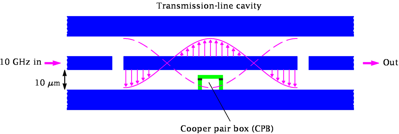 | Fig. 1 (Color online) Schematic of the arrangement to investigate the system. In it a superconducting qubit (green) interacts with the electric field (pink), both inside a transmission line (blue); the latter consists of a central conductor and two ground planes on either side. |
2 Model of the COPB-CQED System

5 ) and Eq. (6 ) in Eq. (7 ) we find the pair of coupled equations,
The CQED is implemented through a transmission line resonator whose electric field is coupled to a superconducting CPB, as shown in Fig.

Thus, we can write the Hamiltonian of the total system in the form,


The state |Ψ(t)⟩ describing the time evolution of the entire system can be written as,
The evolution of the wave function described by Eq. (
3 Evolution of CPB Excitation Inversion and Entropy
The CPB excitation inversion, I(t), here is given by the form,

The entropy SQC(ρQC) is zero when ρQC represents a pure state and is maximum and equal to ln(N) for a state of maximum mixing, where N is the dimension of the Hilbert space. However, here our state is pure only at t = 0; for t > 0 the state of the whole system ceases to be pure due to the presence of losses and the eventual action of time-dependent external fields. Now, concerning the relationship between the entropy 


4 Results and Discussions
4.1 Entropy: (a) Resonant Case
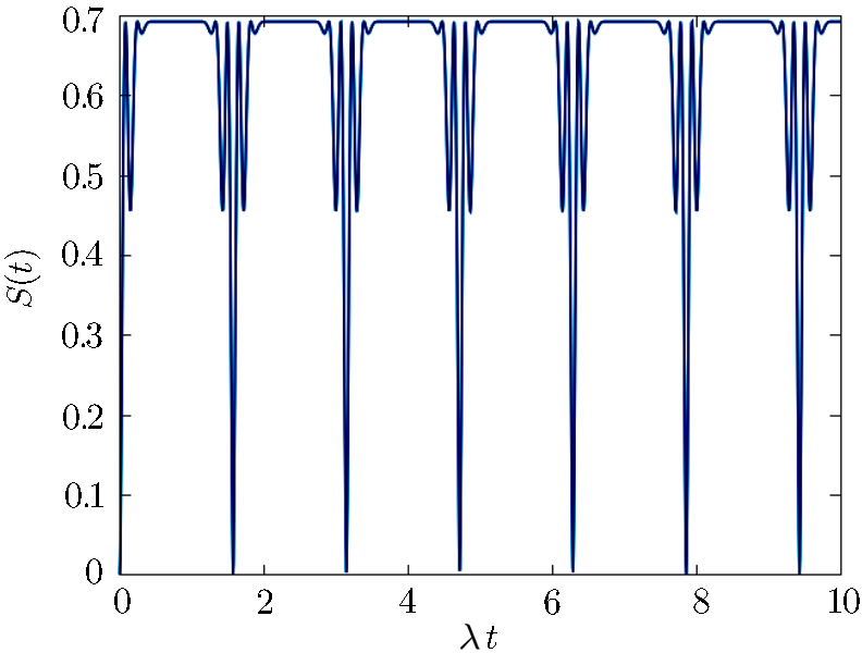
We will initially analyze the entropy of the system in the absence of losses for the superposition of coherent states {|α⟩}, for |α| = 3. Figure
 | Fig. 2 Time evolution of the entropy for the QED-circuit initially in a superposition of coherent states, in the resonant case, for |α| = 3.0, ω0 = 2000λ and ω = 2000λ. |
Figure 
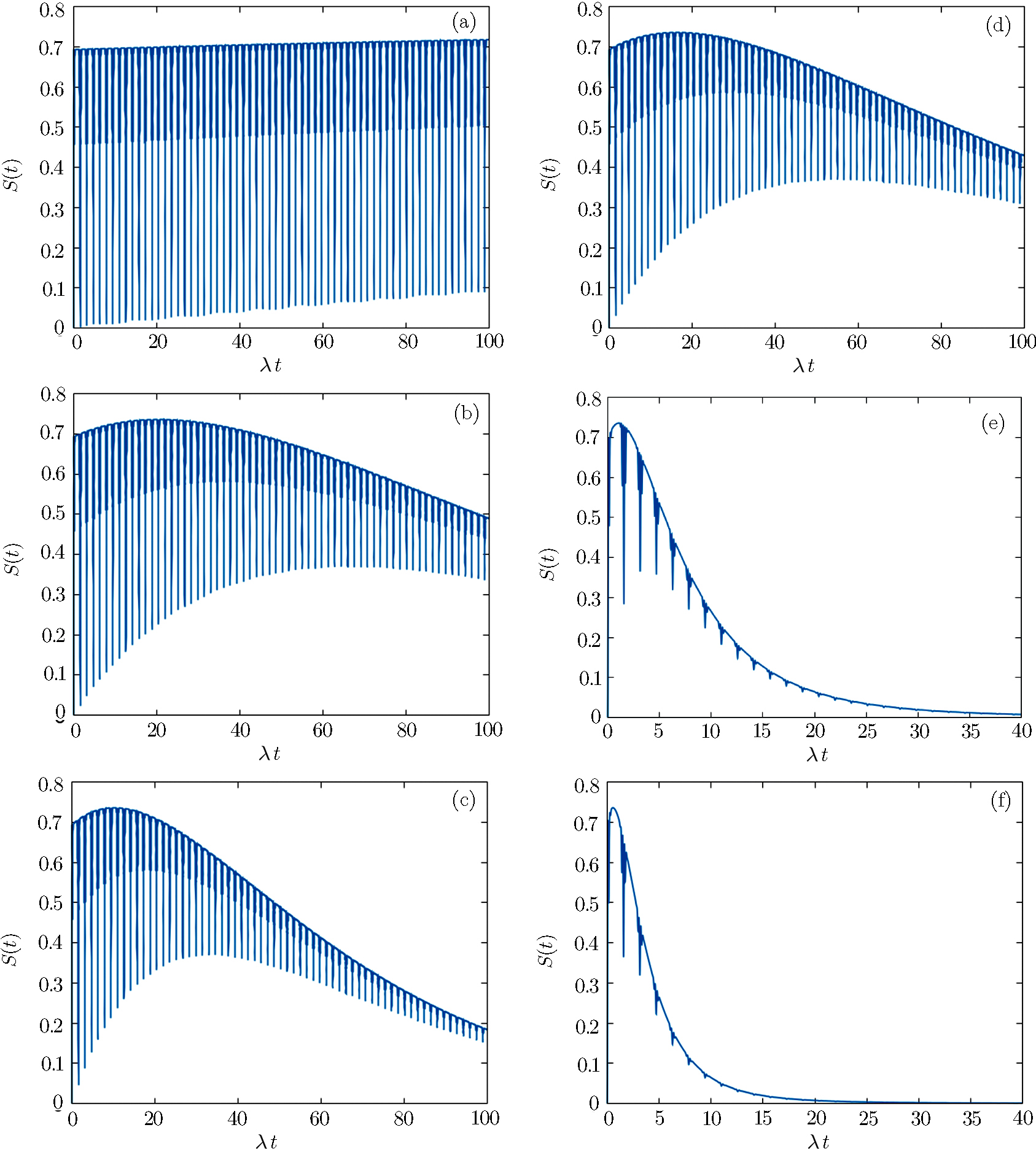
 | Fig. 3 Time evolution of the entropy of the QED-circuit initially in a superposition of coherent states, for |α| = 3.0, ω0 = 2000λ and ω = 2000λ: (a) γ = 0.001λ and δ = 0.0; (b) γ = 0.015λ and δ = 0.0; (c) γ = 0.030λ and δ = 0.0; d) δ = 0.001λ and γ = 0.0; (e) δ = 0.015λ and γ = 0.0; (f) δ = 0.030λ and γ = 0.0. |
Another detail observed is that, for the ratio γ/δ ≈ 16 between the decays the influences on the entropy are quite similar for |α| ≤ 3 (Fig.
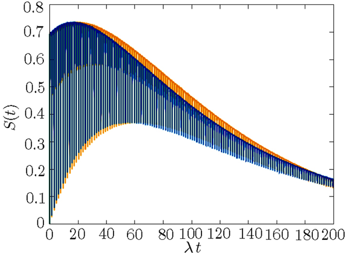
 | Fig. 4 (Color online) Time evolution of the entropy of the QED-circuit initially in a superposition of coherent states, with |α| = 3.0, ω0 = 2000λ and ω = 2000λ. The blue region stands for: γ = 0.0 and δ = 0.001λ; the yellow region is for δ = 0.0 and γ = 0.015λ. |
4.2 Entropy of the System: (b) Non Resonant Case
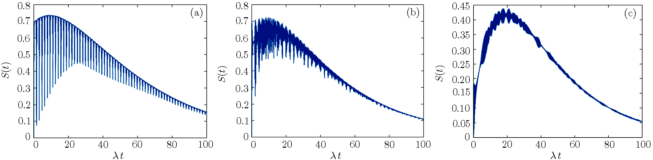
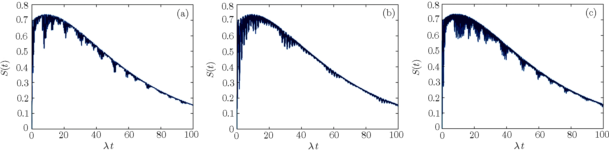
Here the subsystems are assumed non resonant, with fixed detuning f(t) = η. The entropy in absence of loss is smaller than in its presence and the periodicity disappears when detuning increases (Fig.
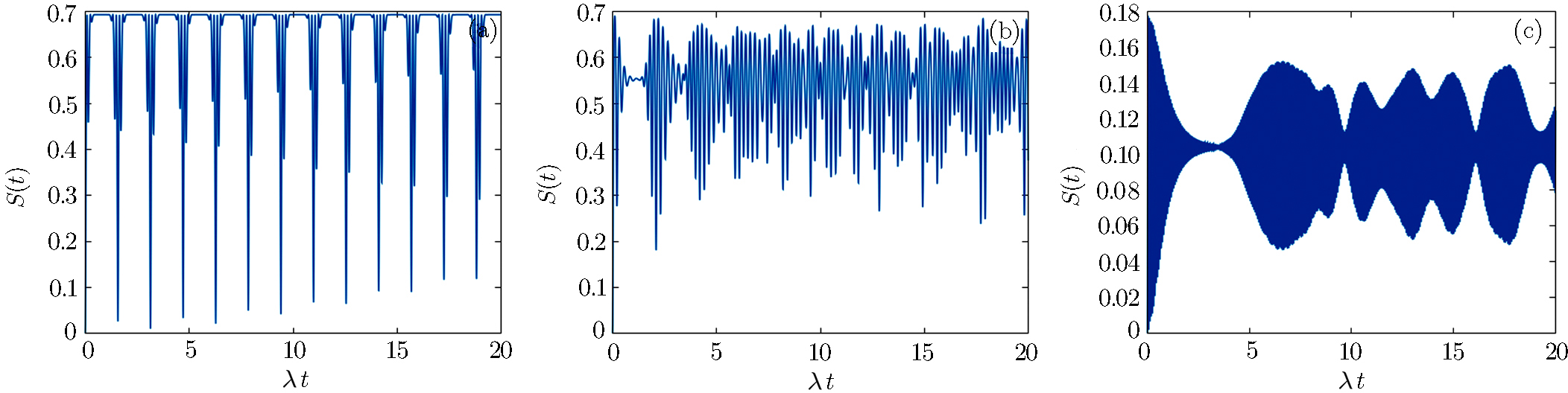 | Fig. 5 Time evolution of the entropy of the QED-circuit initially in a superposition of coherent states, with |α| = 3.0, ω0 = 2000λ, ω = 2000λ, and γ = δ = 0.0; (a) for η = λ; (b) for η = 20λ; (c) for η = 100λ. |
 | Fig. 6 Time evolution of the entropy of the QED-circuit initially in a superposition of coherent states, with |α| = 3.0, ω0 = 2000λ, ω = 2000λ, γ = 0.015λ, and δ = 0.001λ (a) for η = λ; (b) for η = 20λ; (c) for η = 100λ. |
The entropy of the system in presence of losses and a time-dependent detuning (f(t) = η cos(ω′t)) has an opposite effect to what happens when f(t) = η = const. One observes that a variable detuning causes no decrease in the maximum value entropy of the system, as shown in Fig.
 | Fig. 7 Time evolution of the entropy of the QED-circuit initially in a superposition of coherent states, with |α| = 3.0, ω0 = 2000λ, ω = 2000λ, γ = 0.015λ, δ = 0.001λ, and η = 100λ (a) for ω′ = 10; (b) for ω′ = 20; (c) for ω′ = 50. |
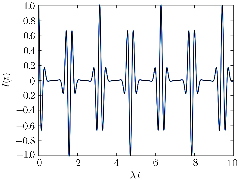
4.3 CPB Excitation Inversion: (a) Resonant Case
Firstly we consider the CPB in absence of losses and the field state in the mentioned superposition of two coherent states, for |α| = 3.0; according to Fig.
 | Fig. 8 Time evolution of the excitation inversion for the QED-circuit initially in coherent state superposition, with |α| = 3.0, ω0 = 2000λ, and ω = 2000λ. |
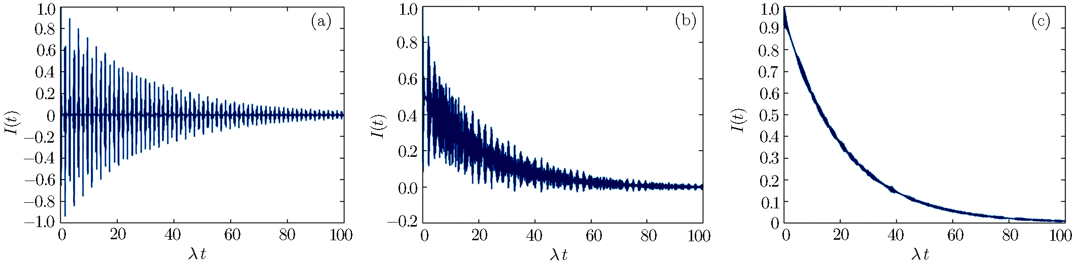
Figure
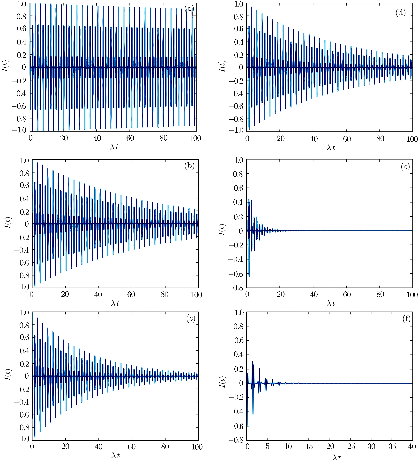 | Fig. 9 Time evolution of the excitation inversion for the QED-circuit initially in coherent state superposition, with |α| = 3.0, ω0 = 2000λ, and ω = 2000λ; (a) for γ = 0.001λ and δ = 0.0; (b) γ = 0.015λ and δ = 0.0; (c) γ = 0.030λ and δ = 0.0; (d) δ = 0.001λ and γ = 0.0; (e) δ = 0.015λ and γ = 0.0; (f) δ = 0.030λ and γ = 0.0. |
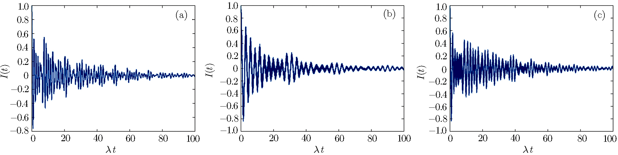
4.4 CPB Excitation Inversion: (b) Non Resonant Case
Here the subsystems are assumed non resonant with constant detuning f(t) = η. The excitation inversion in absence of losses is greater than in their presence and the periodicity disappears when detuning increases (Fig.
 | Fig. 10 Time evolution of the excitation inversion for the QED-circuit initially in coherent state superposition, with |α| = 3.0, ω0 = 2000λ, ω = 2000λ, and γ = δ = 0.0; (a) for η = λ; (b) for η = 20λ; (c) for η = 100λ. |
 | Fig. 11 Time evolution of the excitation inversion for the QED-circuit initially in coherent state superposition, with |α| = 3.0, ω0 = 2000λ, ω = 2000λ, γ = 0.015λ, and δ = 0.001λ; (a) for η = λ; (b) for η = 20λ; (c) for η = 100λ. |
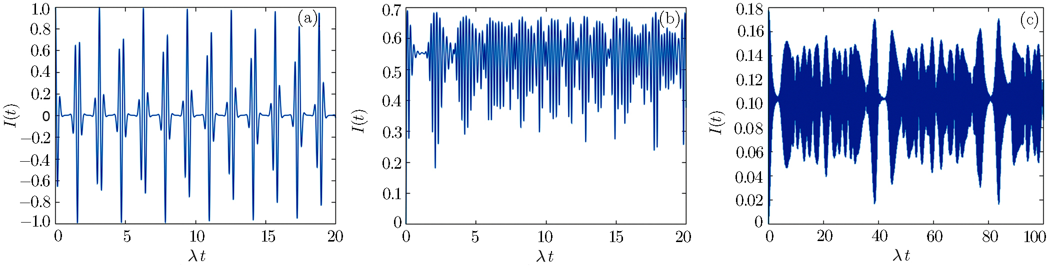
The evolution of excitation inversion of the system in the presence of losses with a variable detuning (f(t) = η cos(ω′t)) shows an opposite behavior to that for f(t) = η = constant. Now the time dependent detuning causes no extinction of the excitation inversion, i.e., the system continues reversing the excitation but maximum value amplitude of inversion decreases with time, as shown in Fig.
 | Fig. 12 Time evolution of the excitation inversion for the QED-circuit initially in coherent state superposition, with |α| = 3.0, ω0 = 2000λ, ω = 2000λ, γ = 0.015λ, δ = 0.001λ, and η = 100λ; (a) for ω′ = 10; (b) for ω′ = 20; (c) for ω′ = 50. |
5 Conclusion
In this work we studied the dynamic properties (entropy of both sub-systems and the CPB excitation inversion) of a hybrid system composed of a CPB and an CQED. We considered the CPB initially excited and the CQED as a superposition of two coherent states. We have assumed the CPB-CQED system described by an intensity-dependent interaction introduced by Buck-Sukumar model. Concerning the entropy, which is related to the entanglement of subsystem states, we studied its time evolution in the presence of losses affecting both subsystems, for resonant and non-resonant cases. The influence on the entropy of a time-dependent (sinusoidal) frequency, via the CQED, was also considered. The excitation inversion was investigated under the same conditions and influences. The inclusion of losses in CPB and CQED makes the scenario more realistic. We have shown that the CQED subsystem is much more sensitive in the presence of losses than the CPB, this can be explained, due to the fact that the CQED presents a much larger number of photons in relation to the CPB. In addition, the time dependence of the coupling λt and CQED frequency ω(t) brings our results to different physical conditions. It was shown that the CPB excitation inversion occurs when detuning is constant in time; however, when it varies the excitation inversion always occurs no matter the value of detuning. In this hybrid system it is possible to control the entropy and inversion of excitation by choosing the parameters appropriately, for example, the appropriate choice of detuning allows us to increase the maximum entropy of the system, which was ∼ 0.45 in Fig.
In summary, it was shown that, when using the intensity-dependent BS model extended to a realistic scenario taking into account influence of losses, detuning and time dependent external fields, interesting results emerge. This also indicates that one can perform a dynamic control of subsystem properties through the manipulation of parameters involved, with potential applications to the command of quantum information processes. We have also shown that the decoherence effect is greater in the CQED, which is due to the fact that the CQED can have more excitations than the CPB. Decoherence affecting the CQED can be reduced by improving its quality. We hope that these results could provide some good insights for researchers in this area.
Reference
| [1] | |
| [2] | |
| [3] | |
| [4] | |
| [5] | |
| [6] | |
| [7] | |
| [8] | |
| [9] | |
| [10] | |
| [11] | |
| [12] | |
| [13] | |
| [14] | |
| [15] | |
| [16] | |
| [17] | |
| [18] | |
| [19] | |
| [20] | |
| [21] | |
| [22] | |
| [23] | |
| [24] | |
| [25] | |
| [26] | |
| [27] | |
| [28] | |
| [29] | |
| [30] | |
| [31] | |
| [32] | |
| [33] | |
| [34] | |
| [35] | |
| [36] | |
| [37] | |
| [38] | |
| [39] | |
| [40] | |
| [41] | |
| [42] | |
| [43] | |
| [44] | |
| [45] | |
| [46] | |
| [47] | |
| [48] |