
Implementation Scheme of Two-Photon Post-Quantum Correlations
Cite this Article
Pan Guo-Zhu, Chu Wen-Jing, Yang Ming, Yang Qing, Zhang Gang, Cao Zhuo-Liang. Implementation Scheme of Two-Photon Post-Quantum Correlations. Communications in Theoretical Physics, 2018, 69(6): 687 
Permissions
Implementation Scheme of Two-Photon Post-Quantum Correlations
† Corresponding author. E-mail:
Supported by National Natural Science Foundation of China (NSFC) under Grant Nos. 11274010, 11374085, and 61370090, Anhui Provincial Natural Science Foundation under Grant Nos. 1408085MA20 and 1408085MA16, the Key Program of Domestic Visiting of Anhui Province under Grant No. gxfxZD2016192
Abstract
Abstract
The pre- and post-selection processes of the “two-state vector formalism” lead to a fair sampling loophole in Bell test, so it can be used to simulate post-quantum correlations. In this paper, we propose a physical implementation of such a correlation with the help of quantum non-demolition measurement, which is realized via the cross-Kerr nonlinear interaction between the signal photon and a probe coherent beam. The indirect measurement on the polarization state of photon is realized by the direct measurement on the phase shift of the probe coherent beam, which enhances the detection efficiency greatly and leaves the signal photon unabsorbed. The maximal violation of the CHSH inequality 4 can be achieved by pre- and post-selecting maximally entangled states. The reason why we can get the post-quantum correlation is that the selection of the results after measurement opens fair-sampling loophole. The fair-sampling loophole opened here is different from the one usually used in the currently existing simulation schemes for post-quantum correlations, which are simulated by selecting the states to be measured or enlarging the Hilbert space. So, our results present an alternative way to mimic post-quantum correlations.
1 Introduction
Quantum systems can have correlations different from those of classical systems. Considering two separated observers, Alice and Bob, sharing a quantum state, each chooses one from a set of possible measurements and obtains some outcomes. In the quantum states with the property of being entangled, Alice and Bob can observe correlations, which cannot be explained by classical models defined in terms of local hidden variables. These non-local correlations can be detected by observing violations of the CHSH inequalities.[1–5] A key feature of nonlocal correlations is that it does not allow the two observers to send information to each other faster than light, i.e., correlations from the measurements on quantum states are non-signaling.
Assuming local realism, the correlations predicted by quantum mechanics cannot violate the CHSH inequality beyond Tsirelson’s bound 
2 Quantum Description of Pre- and Post-Selected Ensembles
Quantum measurement[33–34] plays an essential role in extracting information from a physical system of interest. To observe the post-quantum correlations in quantum systems, pre- and post-selected ensembles must be prepared.[25] That is to say, the generalized description of a quantum system in the time interval between two measurements must be introduced,[23–24] where the generalized state completely describes a quantum system when information about the system is available both from the past and from the future. For a given pre- and post-selected ensemble, suppose the initial state is |ψi⟩ and the final state is |ψf⟩, and thus the probability for an outcome |cn⟩ of an ideal measurement on an observable C at intermediate time is given by ABL formula:[23–24]
3 Implementation of Two-Photon Supercor-relations in Optical System
1 ). Correspondingly, Bob’s projection operators are 
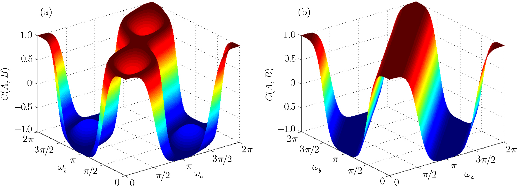
1 , when x = 0, BCHSH = 0, there is no correlation between Alice’s and Bob’s measurements; However, when x > 0, the CHSH inequality can be violated. For example when x = 0.25, ωa = 3π/2, ωa′ = π, ωb = 9π/8, ωb′ = 7π/8, we can get C(A, B) = 0.668, C(A, B′) = −0.668, C(A′, B) = 0.997, C(A′, B′) = 0.997, and thus the CHSH value of the system is 3.33. Furthermore, when x → 0, ωa = 3π/2, ωa′ = π, ωb → π + (approaching π from the right), ωb′ → π − (approaching π from the left), C(A, B) → 1, C(A, B′) → −1, C(A′, B) → 1, C(A′, B′) → 1, so we can obtain the maximal value of the CHSH inequality BCHSH → 4. From the plots in Fig. 1 we can see that the final CHSH values BCHSH vary drastically with the parameters ωa, ωb of the intermediate measurements, but only slightly with the parameter x of the initial and final states. Fortunately, the parameters ωa, ωb of the intermediate measurements can be easily controlled via tuning the angles of the HWPs.
4 ) as
11 ) naturally, that is to say these events are filtered out from the total counting sample, and do not affect the final results of the scheme. But the multi-photon component in Eq. (11 ) can cause the coincidence measurement too, so these events may be included in the total counting sample and introduce errors in the final results. Fortunately, the probability of the multi-photon component is too small γ2 ∼ 10−4,[43–44] which only affects the scheme slightly.
In what follows, we describe in detail how to obtain supercorrelations in pre- and post-selected photon ensembles. Consider a two-photon system whose initial and final states are


For a given system, the CHSH value is defined as BCHSH = |C(A, B) − C(A, B′) + C(A′, B) + C(A′, B′)|,[1] where A and A′ are two-valued (±1) variables for the first system, and B and B′ are similar variables for the second system. The function C(A, B) = PAB(1, 1) + PAB(−1, −1) − PAB(1, −1) − PAB(−1, 1) represents the expected value of A and B for the two systems, and PAB(1, 1) denotes the joint probability of obtaining A = 1 and B = 1 when A and B are measured.
According to the ABL formula (

 | Fig. 1 The correlations C(A, B) are plotted as functions of the parameters of the intermediate measurements ωa, ωb and the parameter x of the initial and final states. (a) x = 0.05, (b) x = 0.25. |
In order to realize two-photon supercorrelations in pre- and post- selected ensembles, three steps are needed, as illustrated in Fig. 


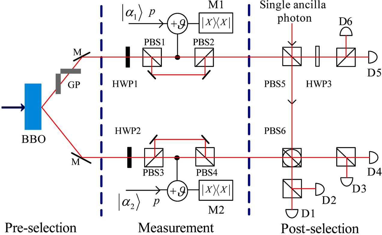 | Fig. 2 Schematic setup for realizing supercorrelations. HWP1 and HWP2 realize the basis transformation | ↑⟩(| ↓ ⟩) ↔ |H⟩(|V ⟩). HWP3 rotates the photon polarization as |H⟩ ↔ sin θ|H⟩ + cos θ|V ⟩, |V ⟩ ↔ −cos θ|H⟩ + sin θ|V ⟩. The + ϑ represents the cross-Kerr nonlinear interaction between the signal photon and the probe coherent beam, where the signal photon will induce a phase shift + ϑ on the coherent beam |α1,2⟩p in the probe mode. |X⟩⟨ X| represents an X quadrature homodyne measurement. PBSi (i = 1, 2, 3, 4, 5) are polarizing beam splitters in {|H⟩, |V ⟩} basis, and PBS6 works in the  |
The second step is to realize the local measurements of the photonic states in the basis of Eq. (

The probe beam is initially prepared in a coherent state, and the interaction between the signal photon and the probe beam will induce a phase shift on the coherent state of the probe beam. Moreover, this phase shift is proportional to the number of the signal photons. The nonlinear interaction between a signal mode and a probe beam can be generally described by the Hamiltonian 


After X quadrature homodyne measurements being performed on the probe beams, the two-photon state will collapse into one of the following four basis states: |HH⟩, |HV⟩, |VH⟩, |VV⟩. Then we can move to the last step—post-selection.
To realize the supercorrelations, the post-selection measurement basis must be chosen as:


Under the above basis, the collapsed two-photon states can be re-expressed as:


In order to post-select the two-photon states, the four two-photon states |φ+⟩, |φ−⟩, |ϕ+⟩, |ϕ−⟩ must be distinguished in this step. To realize this state discrimination process, a PBS, a circular PBS, an HWP, and three photon detectors are needed. The PBS5, circular PBS6 and the HWP3 will transform the joint entangled basis in Eq. (
To understand the relation between the supercorrelations and the measurement outcomes better, we give a brief explanation of how the process realizes the supercorrelations. Assume Alice and Bob share many copies of the pre-selected state |ψi⟩ = sin θ|HH⟩ + sin θ|VV⟩. Firstly, they pick up one copy and perform indirect measurements (M1, M2) of the polarization state of each photon under a certain basis (| ↑a,b⟩, | ↓a,b⟩), and obtain the outcome (x, y), where x = 1 or −1, y = 1 or −1. Then the photons go through PBS5, PBS6 and HWP3. After interacting with an ancilla photon, the two signal photons and the ancilla photon are detected by the detectors D1,D2,D3,D4,D5 and D6. The coincidence measurement among M1, M2, D1, D4, D5 indicates that the measurement outcome (x, y) of the pre- and post-selected state is (|HH⟩), i.e. (1,1). Similarly, the coincidence measurement among M1,D1,D4,D5 indicates the outcome (1, −1), the coincidence measurement among M2,D1,D4,D5 indicates the outcome (−1, 1), and the coincidence measurement among D1,D4,D5 indicates the outcome (−1, −1). The counting rate of (x, y) is proportional to the conditional probability PAB(x, y). To measure other components of the conditional probabilities PA′B(x, y), PAB′(x, y) and PA′B′(x, y), one can rotate the HWP1, 2 by ωa′,b/4, ωa,b′/4 and ωa′,b′/4, respectively. Finally, with the obtained condition probabilities and the expected values, the CHSH value 
In practical experiment, the entanglement source produced by SPDC is not always perfect, which usually generates an entangled state of the form[41–42]

4 Implementation of Two-Photon PR Corre-lations in Pre- and Post-Selected Ensem-bles
We proceed by considering two-photon ensembles with a maximally entangled initial and final state.
The physical realization of the PR correlation includes three steps. Firstly, the maximally entangled bi-photon state 
The set of post-selection measurement basis must be chosen as:
Under the above basis, the two-photon state can be written as:


Thirdly, they verify the final state. The final state |ξ−⟩ will be post-selected as follows. In order to distinguish states |ξ+⟩, |ξ−⟩, |γ+⟩, |γ−⟩ by direct measurements, Alice and Bob need to perform two Hadamard operations and one controlled-not operation 
5 Conclusion
In this paper, we designed an implementation scheme for simulating postquantum correlations by exploiting the fair-sampling loophole in Bell test of bipartite states, which is opened naturally in the “two-state vector formalism” of quantum mechanics without introducing auxiliary Hilbert space, and we can get the probability distributions not only violating CHSH inequality but also surpassing the Tsirelson’s bound. Under the “two-state vector formalism”, the fair-sampling loophole of Bell test is opened by the selection of the results after measurement, which is different from the currently existing simulation schemes for postquantum correlations where the fair-sampling loophole is opened by pre-selecting the states to be measured. Our results verify that the selection of the results after measurement can open fair-sampling loophole too, which can be used to simulate postquantum correlations as well. In addition, our scheme diversifies the simulation tools for postquantum correlations.
In addition, we would like to give an analysis about the feasibility of our simulation scheme. The two challenging building blocks of our scheme are the cross-Kerr nonlinearity in the quantum non-demolition measurement and the Bell state analyzer of the post-selection step. The complete Bell state analyzer needs an optical controlled NOT operation, which has been realized.[40,45–46] Although the success probability of the complete Bell state analyzer is only 1/8 within the current technology, the four Bell states can be completely discriminated with fidelity reaching 89% when it succeeds. Nonetheless, the low success probability of the Bell state analyzer does not affect the current scheme because we only count the events where the coincidence measurement succeeds. On the other hand, the cross-Kerr nonlinearity is still a controversial topic within current technology. One reason is that the natural cross-Kerr nonlinearity is extremely weak, so it is difficult to discriminate the two overlapping coherent states in homodyne detection. Fortunately, some theoretical works have proved that with the help of weak measurement, it is possible to amplify the phase shift induced by single photon to an observable value.[47–48] Recently, the single-photon-level nonlinear phase shift in an optical fibre has been demonstrated experimentally, which uses the photonic crystal fibre as a Kerr medium as it has a high capacity for confining light in its silica core.[49] Of course, there will be errors in the homodyne measurement on coherent probe beams due to the fact that the coherent state |α⟩ and the phase-shifted coherent state of the probe mode are not completely orthogonal, and this error probability is given by 
Reference
| [1] | |
| [2] | |
| [3] | |
| [4] | |
| [5] | |
| [6] | |
| [7] | |
| [8] | |
| [9] | |
| [10] | |
| [11] | |
| [12] | |
| [13] | |
| [14] | |
| [15] | |
| [16] | |
| [17] | |
| [18] | |
| [19] | |
| [20] | |
| [21] | |
| [22] | |
| [23] | |
| [24] | |
| [25] | |
| [26] | |
| [27] | |
| [28] | |
| [29] | |
| [30] | |
| [31] | |
| [32] | |
| [33] | |
| [34] | |
| [35] | |
| [36] | |
| [37] | |
| [38] | |
| [39] | |
| [40] | |
| [41] | |
| [42] | |
| [43] | |
| [44] | |
| [45] | |
| [46] | |
| [47] | |
| [48] | |
| [49] | |
| [50] |