Burgers’ equation is a fundamental partial differential equation, and has gained increasing attention in the study of physical phenomenons in many fields, such as fluid mechanics,^[1] nonlinear acoustics,^[2] traffic flow,^[3] and so on. This equation is originally introduced by Bateman in 1915,^[4] and later in 1947, it is also proposed by Burgers in a mathematical modeling of turbulence,^[5] after whom such an equation is widely used as the Burgers’ equation.

Over past decades, many numerical methods have been proposed to solve Burgers’ equation,^[6–15] including the finite-difference (FD) method,^[6–10] finite-element method,^[11–12] boundary elements method, and direct variational methods.^[13] Actually, these available approaches can be classified into two categories. The first one is to directly solve the nonlinear Burgers’ equation^[14] with the developed numerical methods. However, as pointed out in Ref. [15], in this approach, it is more difficult to balance the convection and the diffusion terms, which usually gives rise to nonlinear propagation effects and the appearance of dissipation layers. To overcome these problems, Cole^[16] and Hopf^[17] introduced the so-called the Cole-Hopf transformation to eliminate the nonlinear convection term in Burgers’ equation, and consequently, the Burgers’ equation can be converted to the linear diffusion equation. Then the second indirect approach, i.e., the Cole-Hopf transformation based method, is also proposed to solve the converted linear diffusion equation.^{[10,13,15,18–19]}

The lattice Boltzmann (LB) method, as a promising technique in computational fluid dynamics, has attracted widespread concern in recent years.^[20–23] Unlike traditional numerical methods, the LB method has some distinct characteristics, including intrinsical parallelism, simplicity for programming, numerical efficiency and ease in incorporating complex boundaries. Except its applications in computational fluid dynamics, the LB method has also been extended to solve some nonlinear partial differential equations,^[24] such as Poisson equation,^[25] wave equation,^[26] diffusion equation,^[27–28] and convection-diffusion equation.^[29–36] Recently, some LB models have been proposed for the Burgers’ equation,^[37–45] however, there are some nonlinear terms in the local equilibrium distribution function,^[37–45] which are more complex and may also generate unstable solution. To overcome the problems inherited in these available LB models for Burgers’ equation, a new Cole-Hopf transformation based LB model would be developed in this work.

The rest of the paper is organized as follows. In Sec. 2, the Cole-Hopf transformation based LB model for Burgers’ equation is proposed. In Sec. 3, some numerical simulations are performed to test present LB model, and finally some conclusions are given in Sec. 4.

In this section, the Burgers’ equation is first linearized by the Cole-Hopf transformation, and then the LB model for converted linear diffusion equation is developed.

We first consider the following one-dimensional Burgers’ equation,

With the help of Cole-Hopf transformation,^[16–17]

And correspondingly, the initial condition (2) and the boundary conditions (3) can be written as

Now, we present an LB model for the linear diffusion equation (5). For simplicity but without losing generality, we only consider a simple D1Q3 (three-discrete velocities in one dimension) lattice model, and three-discrete velocities in this lattice model can be given by

The evolution equation of present LB model reads

It should be noted that discrete velocity c_i and weight coefficient ω_i should satisfy some isotropic constraints,

In the implementation of present LB model, the evolution equation (8) still consists of two steps:

(i) Collision: ,

(ii) Propagation: ,

where is the post-collision distribution function.

We now perform a detailed Chapman-Enskog analysis to derive converted linear diffusion from present LB model. In the Chapman-Enskog analysis, the distribution function, the time and space derivatives can be expended as

Using Eqs. (9), (12) and (13a), we have

Applying Taylor expansion to Eq. (8), one can obtain

Finally, we would like to point out that, after computing ϕ with present LB model, we also need to adopt Eq. (4) to calculate velocity u, and for this reason, some other special methods are also needed to compute ∂_xϕ. Actually in previous studies, the term ∂_xϕ is usually calculated by the traditional nonlocal FD schemes (e.g., Ref. [46]). However in the framework of LB method, it can also be computed by the non-equilibrium part of the distribution function with a second-order convergence rate.^[35–36,47] If we multiply ε on both sides of Eq. (22), and utilize the relation , one can derive an expression for computing ∂_xϕ,

To ensure that the results of ϕ, ∂_xϕ and u are more accurate, we consider the following initialization of distribution function,

In summary, we developed a Cole-Hopf transformation based LB model for Burgers’ equation and the algorithm can be found in the Appendix.

In this section, we conducted several numerical tests to validate present LB model, and to evaluate the accuracy of present model, the following global relative error (GRE) is adopted,

With above initial and boundary conditions, the solution of Eq. (5) can be obtained,^[15]

In our simulations, the computational domain is fixed to be [0,2], and the half bounce-back scheme is adopted for Neumann boundary conditions.^[33,47–48]

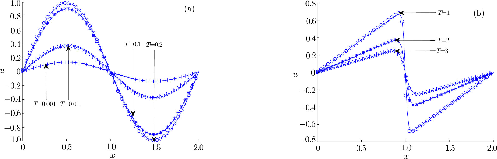
We first carried out some simulations under different diffusion coefficients, and presented the result in Fig. 1. As seen from this figure, the numerical results agree well with the corresponding analytical solutions. Then we also conducted a comparison between present LB model and some existing numerical methods, which are fully implicit finite-difference method (IFDM),^[6] Douglas finite-difference method (DFDM),^[8] B-spline finite element method (BFEM),^[12] local discontinuous Galerkin method (LDG),^[18] a mixed finite difference and boundary element method (BEM)^[49] and Adomian's decomposition method (ADM).^[50] Based on the results listed in Tables 1 and 2, one can find that all numerical results are very close to the exact solutions, while the present model seems more accurate, especially for the case with a large diffusion coefficient.

Fig. 1

	Figure Option ViewDownloadNew Window
	Fig. 1 Numerical and analytical solutions at different time ((a) ν = 1.0, (b) ν = 0.01; solid lines: analytical results, symbols: numerical results).

Table 1

Table 1

Table 1 A comparison between present LB model and some existing numerical methods (ν = 1.0). . Method T x = 0.1 x = 0.3 x = 0.5 x = 0.7 x = 0.9 IFDM[6] 0.1 0.110 09 0.293 35 0.373 42 0.311 44 0.121 28 DFDM[8] 0.109 47 0.291 70 0.371 33 0.309 70 0.120 61 BFEM[12] 0.109 78 0.292 38 0.372 12 0.310 44 0.120 97 LDG(k = 1)[18] 0.109 54 0.291 89 0.371 57 0.309 90 0.120 68 LDG(k = 2)[18] 0.109 54 0.291 89 0.371 57 0.309 90 0.120 69 BEM[49] 0.109 31 0.291 24 0.370 70 0.309 11 0.120 31 ADM[50] 0.109 81 0.292 62 0.372 49 0.310 66 0.120 98 Present 0.109 54 0.291 89 0.371 57 0.309 90 0.120 69 Exact 0.109 54 0.291 90 0.371 57 0.309 91 0.120 69 IFDM[6] 0.2 0.042 37 0.112 76 0.141 20 0.115 74 0.044 57 LDG(k = 1)[18] 0.041 93 0.110 62 0.138 47 0.113 47 0.043 69 LDG(k = 2)[18] 0.041 93 0.110 62 0.138 47 0.113 47 0.043 69 BEM[49] 0.042 20 0.110 44 0.138 09 0.113 22 0.043 91 Present 0.041 93 0.110 62 0.138 47 0.113 46 0.043 69 Exact 0.041 93 0.110 62 0.138 47 0.113 47 0.043 69

Table 1 A comparison between present LB model and some existing numerical methods (ν = 1.0). .

Table 2

Table 2

Table 2 A comparison between present LB model and some existing numerical methods (ν = 0.01). . Method T x = 0.1 x = 0.3 x = 0.5 x = 0.7 x = 0.9 IFDM[6] 0.5 0.121 82 0.362 06 0.590 79 0.794 16 0.933 22 LDG(k = 1)[18] 0.121 10 0.360 16 0.588 61 0.793 63 0.938 67 LDG(k = 2)[18] 0.121 13 0.360 22 0.588 80 0.793 23 0.937 67 BEM[49] 0.120 79 0.361 13 0.595 59 0.812 57 0.971 84 Present 0.121 07 0.360 11 0.588 62 0.792 95 0.933 51 Exact 0.121 14 0.360 27 0.588 70 0.793 49 0.938 11 IFDM[6] 2 0.043 67 0.130 95 0.218 00 0.304 66 0.380 24 LDG(k = 1)[18] 0.042 96 0.128 83 0.214 53 0.299 97 0.373 25 LDG(k = 2)[18] 0.042 96 0.128 83 0.214 55 0.299 98 0.373 25 BEM[49] 0.043 00 0.128 77 0.214 68 0.300 75 0.374 52 Present 0.042 95 0.128 80 0.214 56 0.300 12 0.373 79 Exact 0.042 96 0.128 84 0.214 56 0.300 00 0.373 28 IFDM[6] 4 0.023 64 0.070 92 0.118 17 0.164 99 0.172 26 LDG(k = 1)[18] 0.023 10 0.069 30 0.115 49 0.161 20 0.166 04 LDG(k = 2)[18] 0.023 10 0.069 31 0.115 49 0.161 21 0.166 05 BEM[49] 0.023 24 0.069 35 0.115 50 0.161 25 0.165 15 Present 0.023 10 0.069 29 0.115 48 0.161 22 0.166 17 Exact 0.023 10 0.069 31 0.115 49 0.161 21 0.166 06

Table 2 A comparison between present LB model and some existing numerical methods (ν = 0.01). .

Similarly, with the help of Cole-Hopf transformation, we can also derive the exact solution to Eq. (1),

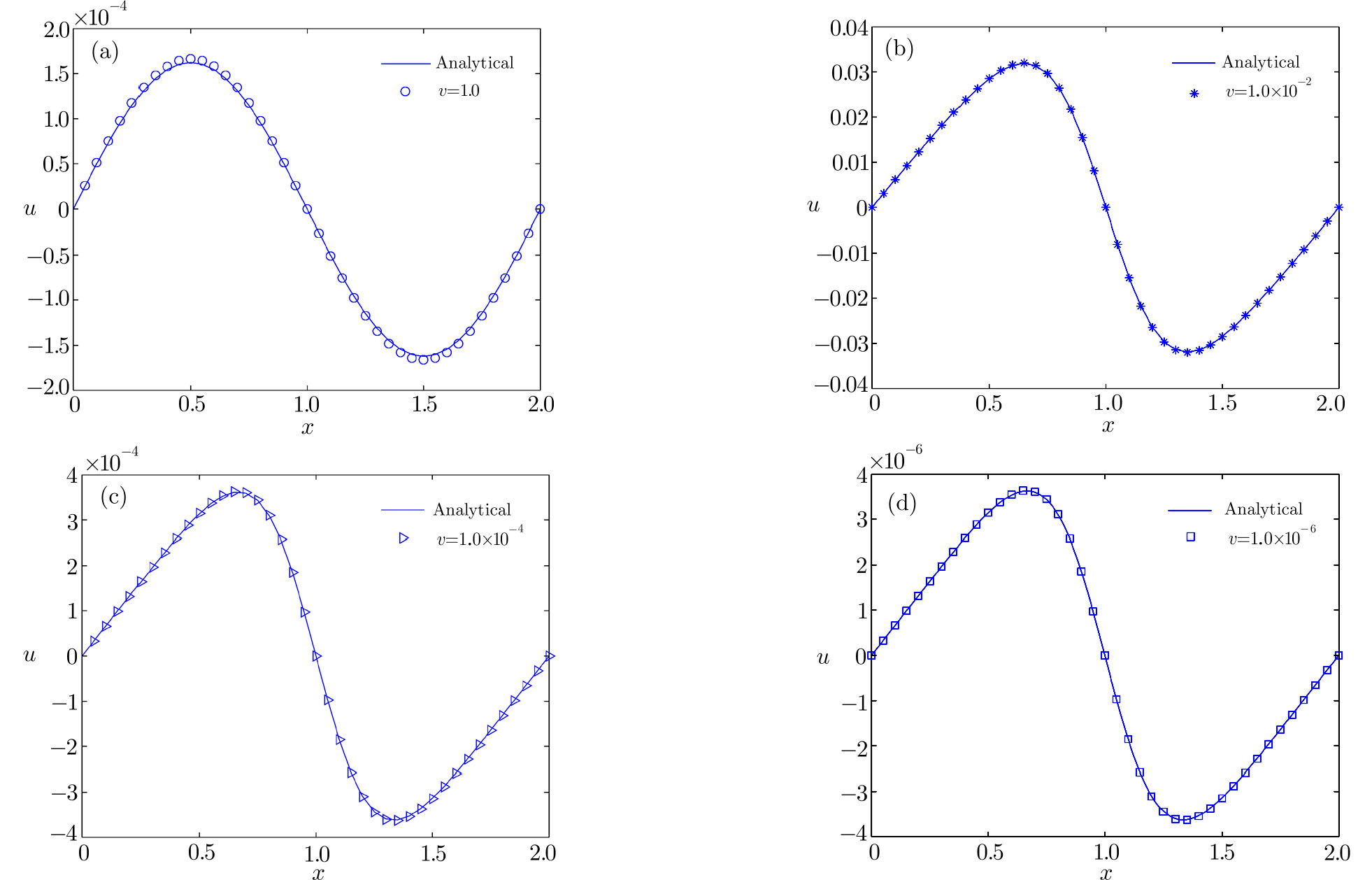
In the following simulations, σ is set to be 2, and the periodic boundary condition is adopted.We first performed some simulations, and presented the results in Fig. 2 where Δx = 0.01, T = 1.0, and ν is varied from 1.0 to 1.0 × 10⁻⁶. From this figure, it is clear that the numerical results are in agreement with the exact solutions. Then a comparison between present LB model and the traditional one^[38] is also conducted, and the results are shown in Table 3 where Δx = 0.025, T = 1.0, and ν is varied from 1.0 to 1.0 × 10⁻³. From this table, one can find that the present LB model is more accurate than the traditional one in solving the Burgers’ equation. Finally, to test the convergence rate of present LB model, we also carried out some simulations, and measured the GREs under different lattice sizes. Based on the results shown in Fig. 3 where ν = 1.0 (1/τ = 0.8) and ν = 0.01 (1/τ = 1.97), we can conclude that the present LB model has a second-order convergence rate in space.

Fig. 2

	Figure Option ViewDownloadNew Window
	Fig. 2 Numerical and analytical solutions under different diffusion coefficients ((a) ν = 1.0, (b) ν = 1.0 × 10−2, (c) ν = 1.0 × 10−4, (d) ν = 1.0 × 10−6; solid lines: analytical results, symbols: numerical results).

Fig. 3

	Figure Option ViewDownloadNew Window
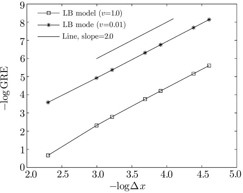
	Fig. 3 GREs of present LB model for Example 2 (Δx = 1/10, 1/20, 1/25, 1/40, 1/50, 1/80, 1/100), the slope of the inserted line is 2.0, which indicates the present LB model has a second-order convergence rate.

Table 3

Table 3

Table 3 GREs of two LB models for Example 2 (Δx = 0.01, T = 1.0). . 1/τ Method ν = 1.0 ν = 1.0 × 10−1 ν = 1.0 × 10−2 ν = 1.0 × 10−3 0.8 Present 3.70 × 10−3 3.90 × 10−5 3.66 × 10−4 4.08 × 10−4 0.8 Ref. [38] 4.10 × 10−3 5.21 × 10−4 4.51 × 10−4 4.92 × 10−4 1.25 Present 1.90 × 10−3 2.00 × 10−5 1.86 × 10−4 2.08 × 10−4 1.25 Ref. [38] 2.20 × 10−3 3.70 × 10−4 2.83 × 10−4 2.60 × 10−4

Table 3 GREs of two LB models for Example 2 (Δx = 0.01, T = 1.0). .

In this paper, a new Cole-Hopf transformation based LB model is proposed for Burgers’ equation. Compared to some available LB models, the present LB model is more accurate since the difficulty and error caused by nonlinear convection term can be avoided. On the other hand, the present LB model is also more efficient since a linear equilibrium distribution function is adopted. In addition, the numerical results also show that the present LB model has a second-order convergence rate in space.

In the next work, we would consider the Cole-Hopf transformation based LB models for two and three-dimensional Burgers’ equations.