

Self-Organized Criticality in an Anisotropic Earthquake Model
Cite this Article
Li Bin-Quan, Wang Sheng-Jun. Self-Organized Criticality in an Anisotropic Earthquake Model. Communications in Theoretical Physics, 2018, 69(3): 280 
Permissions
Self-Organized Criticality in an Anisotropic Earthquake Model
† Corresponding author. E-mail:
Abstract
Abstract
We have made an extensive numerical study of a modified model proposed by Olami, Feder, and Christensen to describe earthquake behavior. Two situations were considered in this paper. One situation is that the energy of the unstable site is redistributed to its nearest neighbors randomly not averagely and keeps itself to zero. The other situation is that the energy of the unstable site is redistributed to its nearest neighbors randomly and keeps some energy for itself instead of reset to zero. Different boundary conditions were considered as well. By analyzing the distribution of earthquake sizes, we found that self-organized criticality can be excited only in the conservative case or the approximate conservative case in the above situations. Some evidence indicated that the critical exponent of both above situations and the original OFC model tend to the same result in the conservative case. The only difference is that the avalanche size in the original model is bigger. This result may be closer to the real world, after all, every crust plate size is different.
1 Introduction
Self-organized criticality (SOC) is a key concept as a possible explanation for the widespread occurrence in many nature systems that long range correlations in space and time.[1–5] Earthquakes are probably the most relevant paradigm of SOC that can be observed by humans on earth. The relevance of SOC to earthquakes was first pointed out by Bak, Tang, and Wiesenfeld,[1] Sornette and Sornette.[6] According to this theory, plate tectonics provides energy input at a slow time scale into a spatially extended, dissipative system that can exhibit breakdown events via a chain reaction process of propagating instabilities in space and time. The empirical Gutenberg-Richter (GR) law[7] arises from the system of driven plates building up to a critical state with avalanches of all sizes. According to the GR law the distribution of earthquake events is scale free over many orders of magnitude in energy.
Then Olami, Feder and Christensen (OFC) introduced a nonconservative model on a lattice that displayed SOC.[8] The OFC model of earthquakes has played an important role in the context of SOC since 1992. However, the presence of criticality in the nonconservative version of the OFC model has been controversial since its introduction and it is still debated.[9–13]
OFC models on different topologies have been investigated in the papers, such as, the annealed random neighbor (ARN) graph model,[14–17] the OFC model on a quenched random (QR) graph[18] and the effects of small-world and scale-free topologies on the criticality of the non-conservative OFC model.[19–24]
Most work in this area is usually focused on their topological properties[25–29] and homogeneous lattices with or without periodic boundary conditions. But the real systems modeled by these objects are not homogeneous. In a geological fault, for example, the local friction between the moving plates, which influences both the rate of motion and the redistribution on the neighbors in the OFC model, cannot be expected to be a constant value but should fluctuate according to local variations. Similarly, the local elasticity of the sheets, which determines how the energy is transferred from one point to another, is also expected to be variable. Therefore, a first step is to simply see how the introduction of quenched disorder in the simple coupled-map representation for these systems will affect their dynamical behavior. Some work has already been done along these lines.
A new earthquake model based on a random network was studied, on which the toppling mechanism of the system is that the force of the unstable site is redistributed to their nearest neighbors randomly.[30–32] It is shown that when the system is conservative, the probability distribution displays power-law behavior. However, it displays no scaling behavior when the system is nonconservative. It is like the results in the ARN OFC model. But it is quite different to the model on quenched random graph[18] and the model on square lattice, both of which display criticality even the system is dissipated. It seems that the toppling mechanism of the system has affected the critical behavior of the system. They also compare the critical behavior of the model with different number of nearest neighbors. It is shown that different spatial topology does not alter the critical behavior of the system.
Mousseau studied the influence of quenched disorder on a coupled map model of earthquakes.[33] In his work, disorder is introduced in the redistribution fraction αi which now varies from site to site as αi = α+δi, where δi is a random number taken from a linear distribution [–δ, δ]. He said that the question of the role of disorder in dynamical systems is fundamental because most biological, neurological, or geological dynamical systems evolve in the presence of one or another type of disorder.
Janosi and Kertesz studied the effect of randomness in the threshold for the OFC rule.[34] They found that this type of disorder destroys criticality and changes the distribution of avalanche size from power law to exponential.
Ceva looked at uncorrelated and correlated disorder in the redistribution parameter α.[35] He was interested, however, in the effects of concentration of defects and not their amplitude. He found that SOC is stable under small concentration of defects.
In this work, we investigate the critical behavior on a modified anisotropic OFC model. Two situations are considered in this paper. One situation is that the energy of the unstable site is redistributed to its nearest neighbors randomly not averagely and keeps itself to zero. The other situation is that the energy of the unstable site is redistributed to its nearest neighbors randomly and keeps some energy for itself instead of reset to zero. Different boundary conditions are considered as well. The rest of the paper is organized as follows. In Sec.
2 Model
The OFC model is defined on a two-dimensional square lattice of L × L sites. Each site is associated a real continuous energy Ei. To mimic that the system is driven continuously and uniformly, the value of Ei increases at the same rate. In simulations, find the largest value of energy Emax in the system and increase the energy of all sites by the same amount Eth − Emax. Therefore, the sites with the largest energy reaches the threshold value (Ei ≥ Eth) and becomes unstable. As soon as a site becomes unstable, i.e., Ei ≥ Eth, the global driving is stopped and the system evolves according to the following local relaxation rule

The toppling of one site triggers an avalanche, that is, neighbors of this site may become unstable and toppling propagates in the network. The avalanche is over until all the sites are below Eth. Then the driving to all sites recovers. The number of toppling sites during an earthquake is defined as the earthquake size S. Open boundary condition is used in OFC model.[36]
Here we modify the OFC model only in the toppling rule: when there is an unstable site toppling, the energy of the site is redistributed to its nearest neighbors randomly not averagely as follows.
If any Ei ≥ Eth then redistribute the energy on Ei to its neighbors randomly according to the following rule
The other model that differs from above model only in the toppling rule: when there is an unstable site, the energy of the site is redistributed to its nearest neighbors randomly and keeps some energy for itself instead of reset to zero, that is not Eqs. (
| Table 1
The different of the two models. . |
To completely define the model, we need to consider the boundary conditions. We care about the open and periodic boundary conditions in our models.[36–39] The energy αE of an unstable site at boundary is lost in the case of open boundary conditions. Periodic boundary conditions mean the energy is not lost, it is transferred to the other side, like a ring. In Table
In a system of SOC, the distribution of earthquake sizes is a power law function. The power-law exponent τ is defined as

3 Simulations and Results
3.1 The One Case of the Modified OFC Model
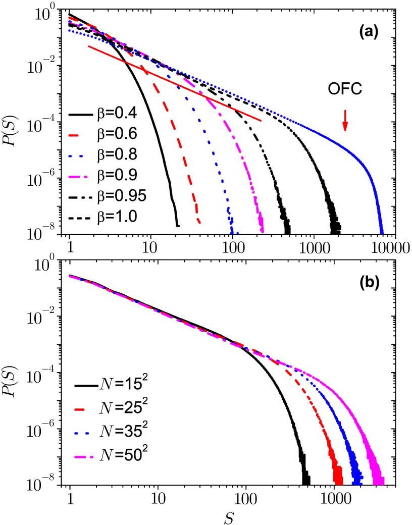
Now we study the one case of the modified OFC model (Case 1). The energy of the unstable site is redistributed to its nearest neighbors randomly not averagely and keeps itself to zero. In comparison to the original OFC model we plot the distribution of avalanche sizes in Fig.
 | Fig. 1 (Color online) Avalanche size distribution with open boundary conditions for (a) different the value of the parameter β with the system size N = 352. Different curves correspond to β = 0.40, 0.60, 0.80, 0.90, 0.95, and 1.0, from left to right. For comparison purposes, the original OFC model of α = 0.25 is shown in the direction of the arrow. (b) Distribution of earthquake size for the different system size with β = 1.0. |
In Fig.
In OFC model, the SOC states exhibit that the distribution is a power law function with an exponential cutoff. The largest avalanche size in OFC model is about 7000. In the modified OFC model, the distribution of avalanche size depends on the dissipation parameter β. The largest avalanche size in modified OFC model is about 1000, which is close to the system size N.
It is not like the result of the original OFC model. The original OFC model exhibits SOC behavior for a wide range of α values and the exponent τ depends on α. However, we find that this modified OFC model exhibits power law distribution when the value of β tends to 1. It is similar with the model on RN[14,16] and small-world networks.[19,23–24]
In Fig.
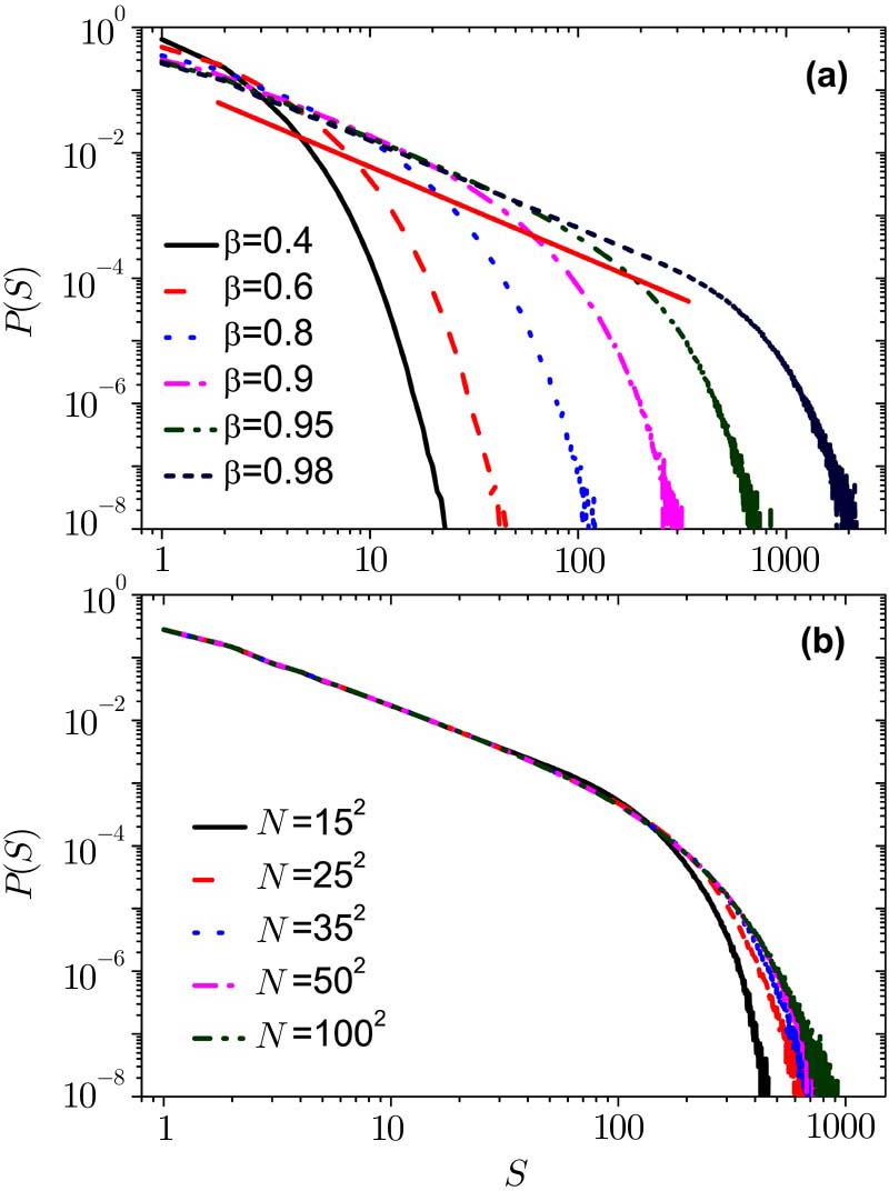
Now we plot the distribution of earthquake size for different values of β with periodic boundary conditions. As shown in Fig.
 | Fig. 2 (Color online) (a) Simulation result for the probability density of having an earthquake of energy E as a function of E for a dissipation parameter β with N = 352 and with periodic boundary conditions. Different curves correspond to β = 0.40, 0.60, 0.80, 0.90, 0.95, and 0.98, from left to right. The fitted curve is shown as red solid line. (b) Distribution of earthquake size for the different system size with β = 0.95. Different curves correspond to N=152, 252, 352, 502, and 1002. |
3.2 The Other Case of the Modified OFC Model
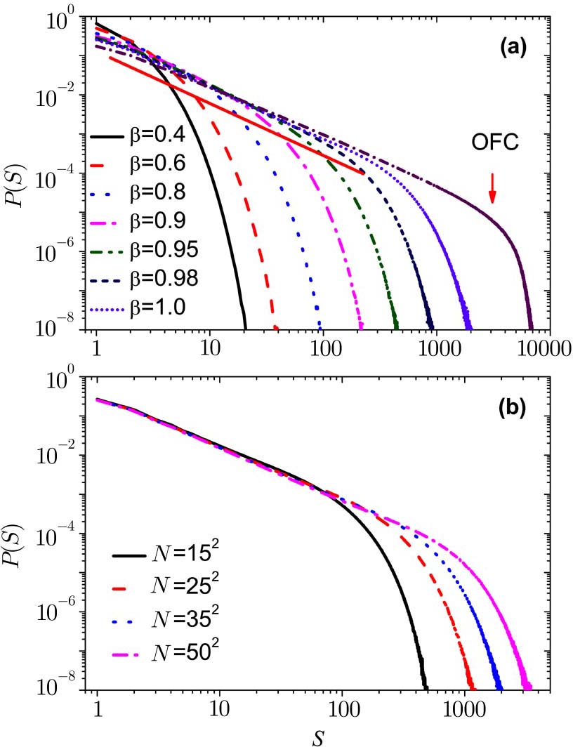
Next, we study the other case of the modified OFC model (Case 2). The energy of the unstable site is redistributed to its nearest neighbors randomly and keeps some energy for itself instead of reset to zero.
In Fig.
 | Fig. 3 (Color online) Avalanche size distribution with open boundary conditions for (a) different the value of the parameter β with the system size N = 352. Different curves correspond to β = 0.40, 0.60, 0.80, 0.90, 0.95, and 1.0, from left to right. For comparison purposes, the original OFC model of α = 0.25 is shown in the direction of the arrow. (b) Distribution of earthquake size for the different system size with β = 1.0. The fitted curve is shown as red solid line. |
The result of this case and the original OFC model tend to the same in the conservative case. The only difference is that the avalanche size in the original model is bigger. This result may be closer to the actual situation, after all, every crust plate size is different.
In Fig.
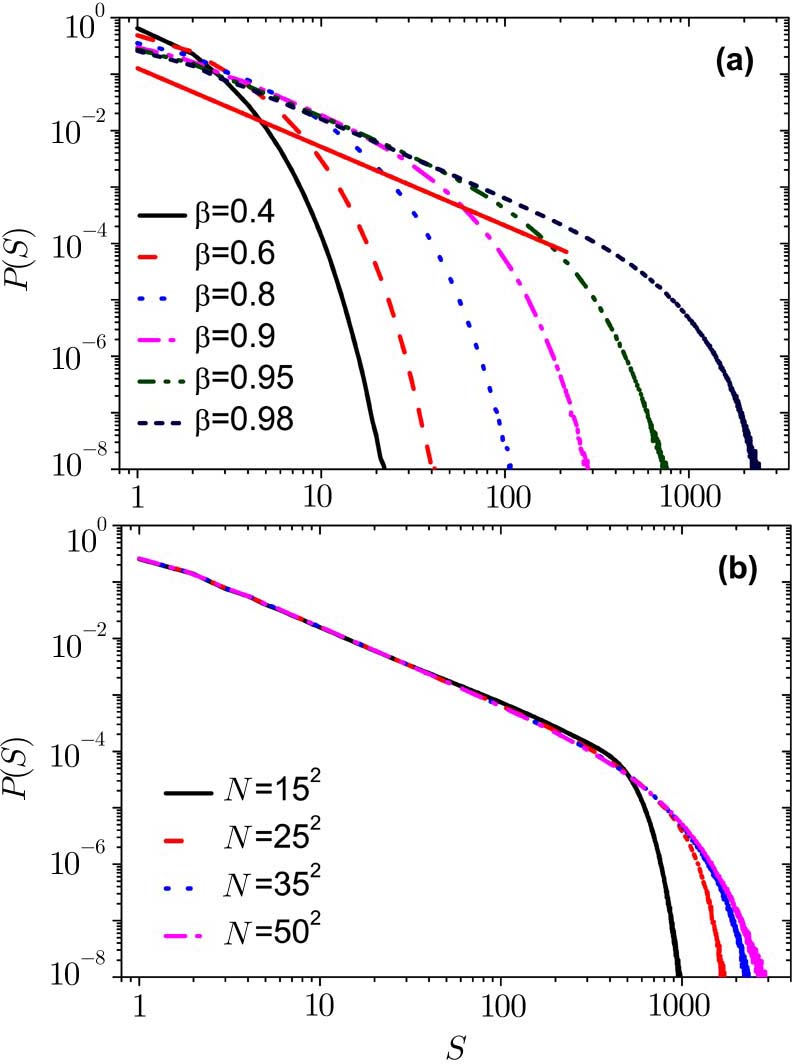
Now we plot the distribution of earthquake size for different values of β with periodic boundary conditions. As shown in Fig.
 | Fig. 4 (Color online) (a) Simulation result for the probability density of having an earthquake of energy E as a function of E for a dissipation parameter β with N = 352 and with periodic boundary conditions. Different curves correspond to β = 0.40, 0.60, 0.80, 0.90, 0.95, and 0.98, from left to right. The fitted curve is shown as red solid line. (b) Distribution of earthquake size for the different system size with β = 0.95. Different curves correspond to N = 152, 252, 352, and 502. |
As shown in Fig.
4 Conclusions
In summary, we have made an extensive numerical study of a modified anisotropic model proposed by Olami, Feder, and Christensen to describe earthquake behavior. The toppling rule is different with that of the OFC model. Two situations were considered in this paper. One case is that the energy of the unstable site is redistributed to its nearest neighbors randomly not averagely and keeps itself to zero. The other case is that the energy of the unstable site is redistributed to its nearest neighbors randomly and keeps some energy for itself instead of reset to zero. Different boundary conditions were considered as well. By analyzing the distribution of earthquake sizes, we found that both above cases can exhibit self-organized criticality only in the conservative case or the approximate conservative case. Some evidence indicated that the critical exponent of both above situations and the original OFC model tend to the same result in the conservative case. The only difference is that the avalanche size in the original model is bigger. It is different from the result of original OFC model. The original OFC model exhibits SOC behavior for a wide range of α values and the exponent τ depend on α. This result may be closer to the real world, after all, every crust plate size is different.
Reference
| [1] | |
| [2] | |
| [3] | |
| [4] | |
| [5] | |
| [6] | |
| [7] | |
| [8] | |
| [9] | |
| [10] | |
| [11] | |
| [12] | |
| [13] | |
| [14] | |
| [15] | |
| [16] | |
| [17] | |
| [18] | |
| [19] | |
| [20] | |
| [21] | |
| [22] | |
| [23] | |
| [24] | |
| [25] | |
| [26] | |
| [27] | |
| [28] | |
| [29] | |
| [30] | |
| [31] | |
| [32] | |
| [33] | |
| [34] | |
| [35] | |
| [36] | |
| [37] | |
| [38] | |
| [39] |