


Fixed-Time Outer Synchronization of Complex Networks with Noise Coupling
Cite this Article
Shi Hong-Jun, Miao Lian-Ying, Sun Yong-Zheng, Liu Mao-Xing. Fixed-Time Outer Synchronization of Complex Networks with Noise Coupling. Communications in Theoretical Physics, 2018, 69(3): 271 
Permissions
Fixed-Time Outer Synchronization of Complex Networks with Noise Coupling
† Corresponding author. E-mail:
Abstract
Abstract
In this paper, the fixed-time outer synchronization of complex networks with noise coupling is investigated. Based on the theory of fixed-time stability and matrix inequalities, sufficient conditions for fixed-time outer synchronization are established and the estimation of the upper bound of the setting time is obtained. The result shows that the setting time can be adjusted to a desired value regardless of the initial states. Numerical simulations are performed to verify the effectiveness of the theoretical results. The effects of control parameters and the density of controlled nodes on the converging time are studied.
1 Introduction
Since being proposed by Pecora and Carroll,[1] synchronization in coupled systems has been extensively studied in many areas, such as biological systems, information processing, economical systems, etc.[2–11] Many kinds of synchronization have been explored, involving complete synchronization,[12] generalized synchronization,[13–14] projective synchronization,[15] and lag synchronization.[16] Due to its widely applications, different control techniques have been constructed, such as adaptive control,[17–19] pinning control,[20] finite-time control,[21–24] sliding mode control,[23,25] and so on.
As a hot research topic, the outer synchronization of complex networks has been extensively investigated.[14,19,26–27] Different from the inner synchronization happening inside a network, outer synchronization is referred as synchronization occurring between two or more networks. In Refs. [14, 27], based on the LaSalle-type invariance principle for stochastic differential equations, the outer synchronization between two nonidentical networks with noise coupling was investigated. The adaptive outer synchronization between two complex delayed networks was discussed in Ref. [19]. Sufficient criterion for outer synchronization between two coupled discrete-time networks were established in Ref. [26].
Most previous works on network synchronization can be divided into two classes: infinite-time synchronization and finite-time synchronization. Finite-time synchronization means that the trajectories of the response system can reach to those of the drive system in a finite horizon, which is very important and significant in the practical engineering process. Because of the fact that the finite settling time is heavily dependent on the initial conditions of the system, it is necessary to obtain the initial states in advance. Nevertheless, the knowledge of initial conditions may be hard to achieve or even impossible to estimate in practical applications. To overcome this obstacle, a new approach named fixed-time control has been proposed.[20,28–34]
Fixed-time control implies that the system is globally finite-time stable and the convergence settling time is bounded and independent of the initial states. Thus, this new technique has important practical implications. For example, to ensure excellent power supply quality and avoid voltage collapse, we should eliminate the frequency deviation and stabilize the voltage of power systems to its nominal value within a limited time. In Ref. [29], for chaos suppression and voltage stabilization in some three-bus power systems, a fixed-time sliding mode control approach was proposed. To realize the finite-time and fixed-time cluster synchronization, Liu and Chen designed simple distributed protocols with or without pinning control.[30] For a class of delayed memristor-based recurrent neural networks, Cao and Li established sufficient conditions of fixed-time synchronization.[31] Hong et al. found that fixed-time control protocols can guarantee any prescribed convergence time regardless of the initial states.[32] In Ref. [33], for fixed-time stabilization of single-input and multi-input systems, Polyakov proposed two different types of nonlinear controller. Based on the Lyapunov methods, a fixed-time terminal sliding-mode control technique for the second-order nonlinear systems was investigated in Ref. [34]. To our best knowledge, there are few results on the fixed-time outer synchronization of complex networks with noise coupling. Actually, noise may play an important role on the collective dynamics of complex systems,[35] which inspired us to study the effect of noise on the fixed-time outer synchronization.
In this paper, based on the theory of fixed-time stability and matrix inequalities, sufficient conditions for the fixed-time outer synchronization of complex networks with noise coupling are presented. The theoretical results show that the setting time can be adjusted to a desired value regardless of the initial states. To verify the effectiveness of the proposed synchronization scheme, numerical simulations are performed.
The rest of this paper is organized as follows. In Sec.
2 Network Modeling and Preliminaries1 ) and (2 ), ui(t) (i = 1, 2, . . ., N) are the controllers to be designed. The noise term in system (2 ) is often used to describe the coupling process influenced by many factors, such as inaccurate design of coupling strength and environmental fluctuation. Here σi : Rn → Rn × s is the noisy intensity matrix, W = (w1, . . ., ws)T is an s-dimensional Brownian motion defined on a complete probability space 

D = (dij)N×N is the coupling configuration matrix, which is similar to the definition of matrix C , ei(t) = yi(t) − ϕ(xi(t)) is the generalized synchronization error between networks (1 ) and (5 ), ϕ : Rn → Rn is a given continuously differentiable map and ϕ(xi) = (ϕ1(xi), ϕ2(xi), . . ., ϕn(xi))T. The controllers ui(t) in Eq. (5 ) are to be designed.


6 ) has a unique and global solution denoted by 
6 ).
Consider a complex network consisting of N nodes with linear couplings:
In order to achieve the fixed-time outer synchronization between complex networks with noise coupling, we refer to model (
In order to get our main results in the next section, we state here some needed concepts, assumptions and lemmas.
To achieve the complete outer synchronization in fixed time, we design
From Eqs. (
In fact, if we consider the outer synchronization between two different networks, both the topological structure and the node dynamics may be different. The response network can be restructured as follows:
Since the speed of the environmental fluctuations is much less than the change rate of concrete systems,[18,27,36–38] for the noise intensity function, we have the following assumption:
Moreover, σ(0) ≡ 0.
For the n-dimensional stochastic differential equation:[39]

For each V ∈ C2,1(Rn × R+, R+), the operator 
3 Main Results
3.1 Fixed-Time Complete Outer Synchronization1 , we can get the conclusion and the fixed settling time T0 can be estimated as Eq. (8 ). This completes the proof of Theorem 1 .
Using matrix transpose properties, one has

By Lemma
Thus

If 

From the Itô formula, we have
Taking the expectations on both sides of Eq. (
3.2 Fixed-Time Generalized Outer Synchronization1 , we obtain
1 and is therefore omitted.
The fixed-time complete outer synchronization can not be achieved if two networks have different dynamics. In the following, we consider the generalized outer synchronization between networks (
By Eq. (

Note that

If 

4 Numerical Simulations
In this section several numerical results are given to verify the effectiveness of the theoretical results. In the simulations, the Euler-Maruyama numerical scheme[42] for stochastic differential equations was used. Without loss of generality, we take the inner coupling matrix
4.1 Numerical Example of Complete Synchronization
We take the Rössler-like system as the node dynamics of networks (
As shown in Fig.
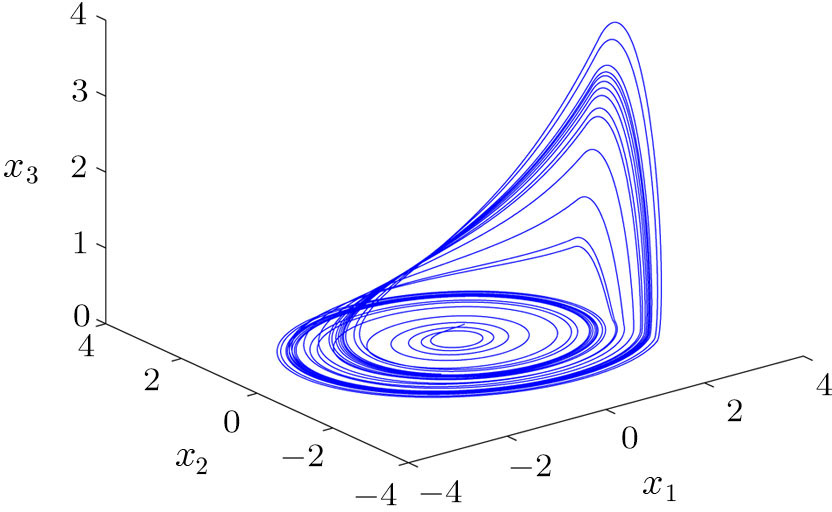 | Fig. 1 Chaotic attractor generated by the system ( |
Let 
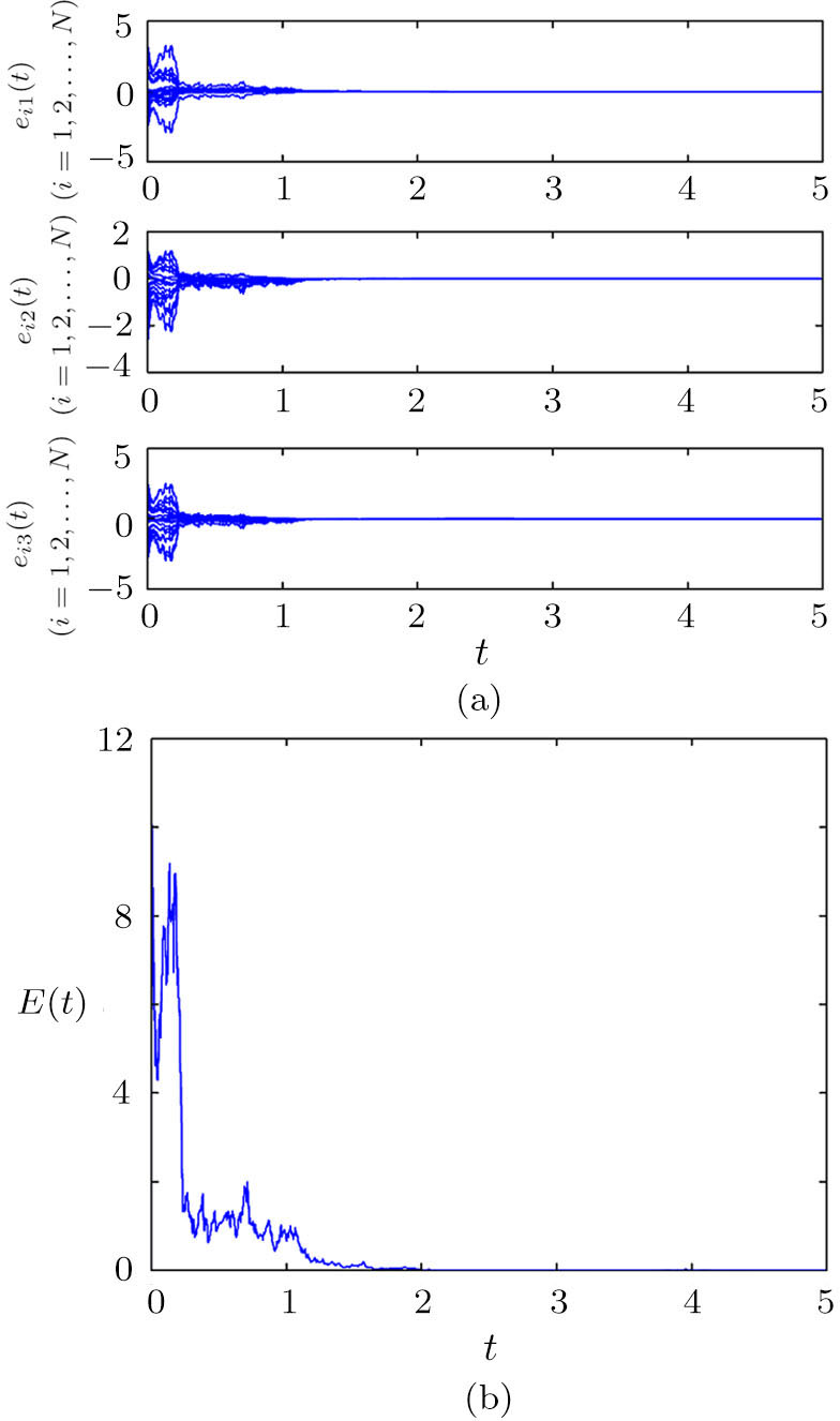
For brevity, taking N = 100 and σ0 = 1.9, we simulate the evolution of the networks according to the controllers defined in Eq. (
 | Fig. 2 Trajectories of the synchronization error (a) and the total synchronization error (b) between networks ( |
Compared with finite-time synchronization, the settling time of fixed-time synchronization is bounded and independent of the initial states. Figure
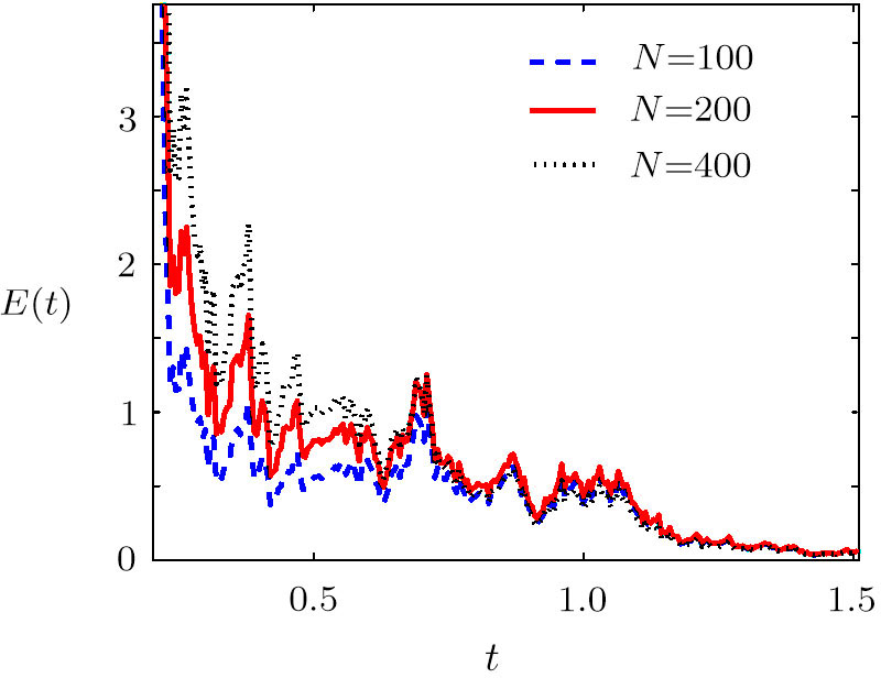
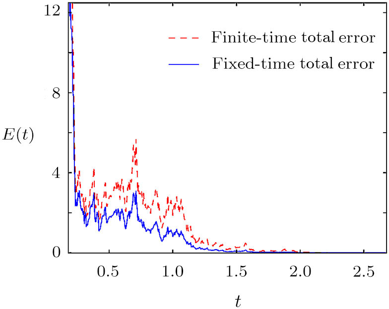 | Fig. 3 Trajectories of the total synchronization error between networks ( |
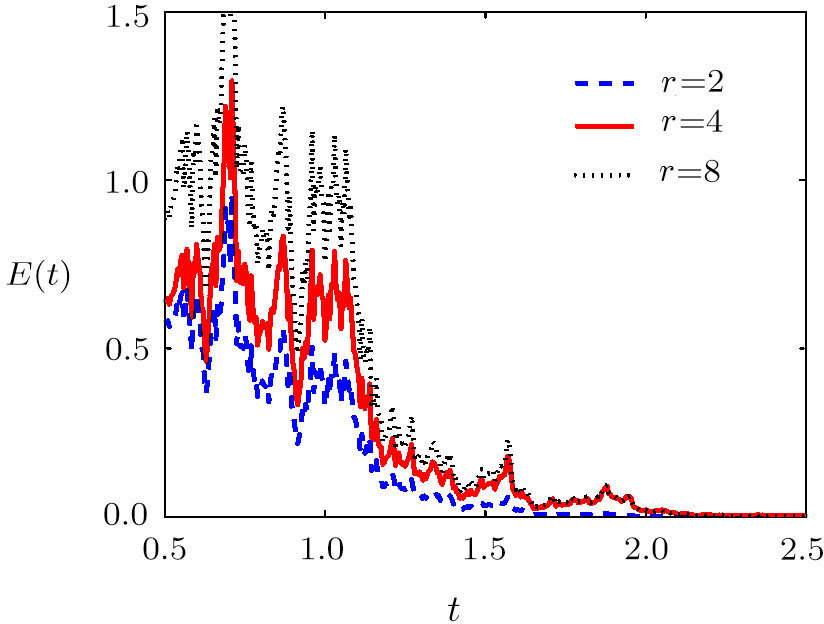
 | Fig. 4 Trajectories of the total synchronization error between networks ( |
To obtain a more accurate estimation of T0, we can appropriately adjust the parameter γ of the controller (
 | Fig. 5 Trajectories of the total synchronization error between networks ( |
Actually, the fixed-time synchronization of complex networks may be achieved without controlling all the network nodes. In fact, many complex networks contain large number of nodes, taking all nodes under control is high-cost and difficult to implement. Therefore, pinning control scheme,[16,20,30,44] which only needs a small fraction of nodes to be controlled, is more suitable to control complex networks to reduce computational burden and equipment resource. The effects of choosing different pinning schemes (high-degree, low-degree and random) on the convergence speed are exhibited in Fig.
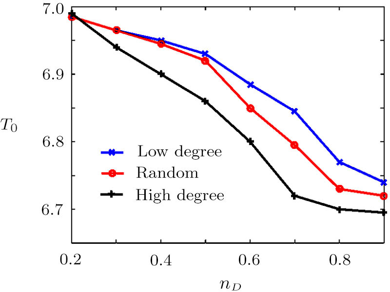 | Fig. 6 The effect of different pinning schemes on the convergence indicator of Scale-free networks with N = 400, σ0 = 1.9, k = 0.6, c1 = 0.1, c2 = 0.2, θ1 = 0.5, θ2 = 1.5. |
4.2 Numerical Example of Generalized Synchronization
To demonstrate the effectiveness of Theorem
Let the continuously differentiable map ϕ : R3 → R4 be

For brevity, taking N = 100 and σ0 = 1.9, we also take
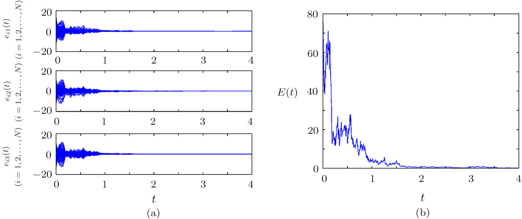
 | Fig. 7 Trajectories of the fixed-time generalized synchronization error (a) and the total generalized synchronization error (b) between networks ( |
5 Conclusion
In this paper, we have investigated the fixed-time outer synchronization between complex networks with noise coupling. Based on the fixed-time control method and inequality techniques, sufficient conditions of fixed-time outer synchronization are proposed. The theoretical analysis indicates that the upper bound of convergence time is determined by the network size N. To verify the effectiveness of the proposed synchronization scheme, for a given scale-free network, numerical simulations are performed and the effects of different pinning schemes on the convergence rate are analyzed. Compared with finite-time synchronization, the settling time of fixed-time synchronization is bounded and independent of the initial states, and thus, has a better performance. Note that time delay may influence the dynamic behavior of complex networks, the fixed-time outer synchronization of time-delayed complex networks is our future direction.
Reference
| [1] | |
| [2] | |
| [3] | |
| [4] | |
| [5] | |
| [6] | |
| [7] | |
| [8] | |
| [9] | |
| [10] | |
| [11] | |
| [12] | |
| [13] | |
| [14] | |
| [15] | |
| [16] | |
| [17] | |
| [18] | |
| [19] | |
| [20] | |
| [21] | |
| [22] | |
| [23] | |
| [24] | |
| [25] | |
| [26] | |
| [27] | |
| [28] | |
| [29] | |
| [30] | |
| [31] | |
| [32] | |
| [33] | |
| [34] | |
| [35] | |
| [36] | |
| [37] | |
| [38] | |
| [39] | |
| [40] | |
| [41] | |
| [42] | |
| [43] | |
| [44] |