


Discrete Boltzmann Method with Maxwell-Type Boundary Condition for Slip Flow
Cite this Article
Zhang Yu-Dong, Xu Ai-Guo, Zhang Guang-Cai, Chen Zhi-Hua. Discrete Boltzmann Method with Maxwell-Type Boundary Condition for Slip Flow. Communications in Theoretical Physics, 2018, 69(1): 77 
Permissions
Discrete Boltzmann Method with Maxwell-Type Boundary Condition for Slip Flow
† Corresponding author. E-mail:
Abstract
Abstract
The rarefied effect of gas flow in microchannel is significant and cannot be well described by traditional hydrodynamic models. It has been known that discrete Boltzmann model (DBM) has the potential to investigate flows in a relatively wider range of Knudsen number because of its intrinsic kinetic nature inherited from Boltzmann equation. It is crucial to have a proper kinetic boundary condition for DBM to capture the velocity slip and the flow characteristics in the Knudsen layer. In this paper, we present a DBM combined with Maxwell-type boundary condition model for slip flow. The tangential momentum accommodation coefficient is introduced to implement a gas-surface interaction model. Both the velocity slip and the Knudsen layer under various Knudsen numbers and accommodation coefficients can be well described. Two kinds of slip flows, including Couette flow and Poiseuille flow, are simulated to verify the model. To dynamically compare results from different models, the relation between the definition of Knudsen number in hard sphere model and that in BGK model is clarified.
1 Introduction
In recent years, the development of natural science and engineering technology has moved towards miniaturization. One of the most typical examples is Micro-Electro-Mechanical System (MEMS).[1–4] It is extremely important to investigate the underlying physics of unconventional phenomena at the micro-scale. Those unconventional phenomena cannot be explained by the traditional macro-model and has become a key bottleneck limiting the further development of MEMS. Among these unconventional physical problems, the gas flow and heat transfer characteristics at the mico-scale are especially critical.
Due to the reduction of the geometric scale, the mean free path of gas molecules may be comparable to the length scale of the device. The Knudsen number (Kn), a dimensionless parameter used to measure the degree of rarefaction of the flow and defined as the ratio of the mean free path of molecules to characteristic length of the device, may be larger than 0.001 and reaches slip-flow regime (

In practical, gas flow in a microchannel may encounter continuum, slip and transition regimes simultaneously. Traditionally macro-scale models cannot apply to such a broad range of Knudsen numbers by only one set of equations. Besides, the numerical solutions of higher order macro-equations are difficult to obtain because of the numerical stability problem.[3] It is commonly accepted that Direct Simulation Monte Carlo (DSMC)[4,8] is an accurate method for rarefied gas flow, which has been verified by experimental data. However, the computation cost in numerical simulations is too expensive for low speed gas flow. To reduce the huge ratio of the noise to the useful information, extremely large sample size is needed. Although, the information preservation (IP) method was presented to treat this problem,[9] the contradiction between the noise problem and sample size has not been well solved.
It has been know that rarefied gas dynamics are represented properly by the Boltzmann equation due to its kinetic nature. That is continuum, slip and transition regimes can be described by one equation. Unfortunately, the Boltzmann equation is a 6-dimensional problem and the computational cost is formidable to solve such an equation by numerical method directly. In order to alleviate the heavy computational burden of directly solving Boltzmann equation, a variety of Boltzmann equation-based methods, such as the unified gas-kinetic scheme (UGKS),[10–11] the discrete velocity method (DVM),[12] the discrete unified gas-kinetic scheme (DUGKS),[13–14] the lattice Boltzmann method (LBM),[2,15–26] have been presented and well developed. Recently, Discrete Boltzmann Method (DBM) has also been developed and widely used in various complex flow simulations,[27–29] such as multiphase flows,[30] flow instability,[31–32] combustion and detonation,[33–34] etc. From the viewpoint of numerical algorithm, similar to finite-different LBM, the velocity space is substituted by a limited number of particle velocities in DBM. However, the discrete distribution function in DBM satisfies more moment relations, which make it fully compatible with the macroscopic hydrodynamic equations including energy equation. The macroscopic quantities, including density, momentum, and energy are calculated from the same set of discrete distribution functions. From the viewpoint of physical modeling, beyond the traditional macroscopic description, the DBM presents two sets of physical quantities so that the nonequilibrium behaviors can have a more complete and precise description. One set includes the dynamical comparisons of nonconserved kinetic moments of distribution function and those of its corresponding equilibrium distribution function. The other includes the viscous stress and heat flux. The former describes the specific nonequilibrium flow state, the latter describes the influence of current state on system evolution. The study on the former helps understanding the latter and the nonlinear constitutive relations.[35] The new observations brought by DBM have been used to understand the mechanisms for formation and effects of shock wave, phase transition, energy transformation, and entropy increase in various complex flows,[30,34,36] and to study the influence of compressibility on Rayleigh–Taylor instability.[31–32] In a recent study, it is interesting to find that the maximum value point of the thermodynamic nonequilibrium strength can be used to divide the two stages, spinnodal decomposition and domain growth, of liquid-vapor separation.
Some of the new observations brought by DBM, for example, the nonequilibrium fine structures of shock waves, have been confirmed and supplemented by the results of molecular dynamics.[37–39] It should be pointed out that the molecular dynamics simulations can also give microscopic view of points to the origin of the slip near boundary, such as the non-isotropic strong molecular evaporation flux from the liquid,[40] which might help to develop more physically reasonable mesoscopic models for slip-flow regime.
In order to extend DBM to the micro-fluid, it is critical to develop a physically reasonable kinetic boundary condition. Many efforts have been made to devise mesoscopic boundary condition for LBM to capture the slip phenomenon.[2,22–26] However, the previous works are most suitable for two-dimensional (2D) models with a very small number of particle velocities and can not be directly applicable to the DBM. On the other hand, those boundary conditions fail to capture flow characteristics in the Knudsen layer so the effective viscosity or effective relaxation time approach needs to be adopted.[15,19] Besides, the results of LBM and DBM should be verified by the results of continuous Botlzmann equation. In 2009, Watari[16] gave a general diffuse reflection boundary for his thermal LB model[41] and investigated the velocity slip and temperature jump in the slip-flow regime. Then, in his sequent work,[42] he compared the relationship between accuracy and number of particle velocities in velocity slip. Two types of 2D models, octagon family and D2Q9 model, are used. It was found that D2Q9 model fails to represent a relaxation process in the Knudsen layer and the accuracy of the octagon family is improved with the increase in the number of particle velocities. However, all the boundary conditions were set as diffuse reflection wall and the tangential momentum accommodation coefficient (TMAC) was not taken into account.
Because of the dependence of the mean free path on microscopic details of molecular interaction, especially the collision frequency, the Knudsen number may have different values in various interaction models for the same macroscopic properties.
In this paper, we first clarify the definitions of Knudsen number and the connection between the hard sphere model and BGK model for three-dimensional (3D) condition so that the results obtained from various models can be compared dynamically. Then a general Maxwell-type boundary condition for DBM is represented and accommodation coefficient is introduced to implement a gas-surface interaction model. Two kinds of gas flows, Couette flow and Poiseuille flow, in a microchannel are simulated. In the section of Couette flow, the relation between the analysis solutions based on hard sphere and BGK model are verified. The simulation results with various Knudsen numbers and accommodation coefficients are compared with analytical ones based on linear Boltzmann equation in the literature not only on the velocity slip but on the Knudsen profiles. While in the section of Poiseuille flow, the simulation results are compared with analytical solution based on Navier–Stokes equation and the second order slip boundary condition.
2 Models and Methods
2.1 Definition of Knudsen Number


4 ) and Eq. (8 ) yields the relationship between viscosity-based mean free path 

The Knudsen number is defined as the ratio of the free path of molecules (λ) to the characteristic length (L),
For the hard sphere collision model, the molecules are considered as hard spheres with diameter d, the mean free path of molecules 
For the BGK model, the mean free path of molecules 

According to the kinetic theory of gas molecules, 

2.2 Discrete Boltzmann Model


The 3D discrete Boltzmann model taking into account the effect of the external force was presented based on the thermal model represented by Watari.[41] The evolution of the discrete distribution function fki for the velocity particle 
To recover the NS equations, the local equilibrium distribution function should retain up to the fourth order terms of flow velocity. The discrete local equilibrium distribution 
The velocity particles 
| Table 1
Discrete velocity model, where |
The Fk in Eq. (


2.3 Boundary Condition Models1 ) is calculated by

17 ) with Eq. (18 ) is applied from the left wall to the node 


To solve the evolution equation (
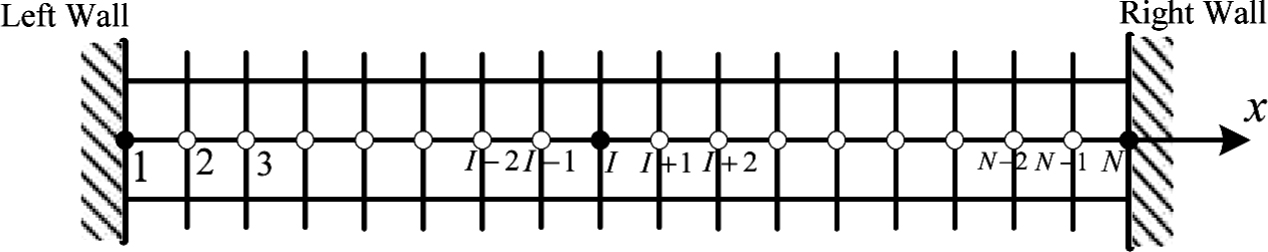 | Fig. 1 Schematic of the space grid. |
For 
To solve the value of the distribution function on the left wall for 

(i) Diffuse reflection boundary
The complete diffuse reflection model assumes that the molecules leaving the surface with a local equilibrium Maxwellian distribution irrespective of the shape of the distribution of the incident velocity. It can be expressed as


The equilibrium distribution functions, 
As a result, the distribution function on the left wall (


(ii) Specular reflection boundary
The specular reflection model assumes that the incident molecules reflect on the wall surface as the elastic spheres reflect on the entirely elastic surface. The component of the relative velocity normal to the surfaces reverses its direction while the components parallel to the surface remain unchanged. As an example, the direction normal to the wall surface parallels to the x axis, then the molecules leave the surface with a distribution as
Since the distribution function 


(iii) Maxwell-type boundary
In practice, the real reflection of molecules on the body surfaces cannot be described properly by complete diffuse reflection or pure specular reflection. So the Maxwell-type reflection model which is composed of the two reflection modes is needed. The TMAC, α is introduced to measure the proportion of complete diffuse reflection.[4] The α portion of the incident molecules reflect diffusely and the other (
Under this boundary condition, the distribution function on the right wall, (


3 Simulation Restlts
3.1 Couette Flow


30 ) and Eq. (31 ) since 


2 . It should be noted that 

3 when 
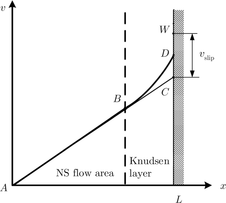
Consider a gas flow between two parallel walls, one at 


The typical velocity profile between parallel plates in the slip-flow regime is depicted in Fig. 


 | Fig. 2 Schemtic of typical velocity profile for Couette flow with slip effect (right half). |
For the hard sphere model,
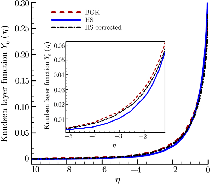
Knudsen profile 

The Knudsen layer function for hard sphere model, 


 | Fig. 3 Profiles of the function  |
Considering the Maxwell-type boundary condition, Onishi[45] gave the expression of slip velocity and Knudsen layer function 
| Table 2
Coefficients for several kinds of values of α. . |
The DBM simulation results for the Couette flow with different Knudsen numbers under complete diffusion boundary condition are shown in Fig.
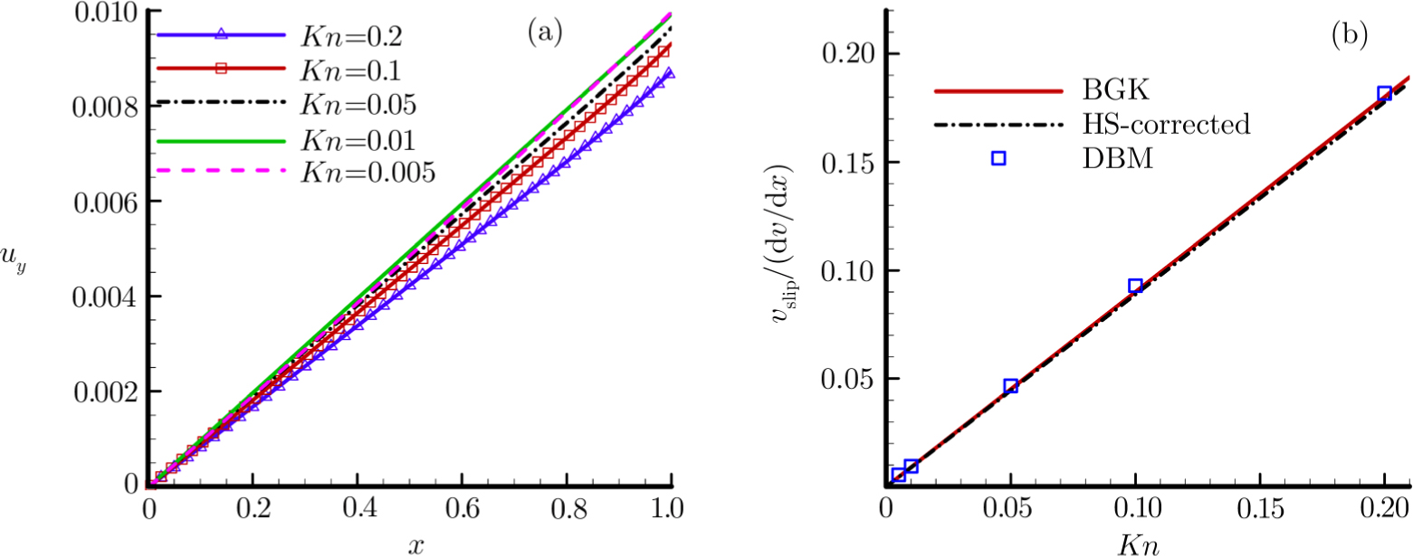 | Fig. 4 DBM simulation results for different Knudsen numbers under complete diffusion reflection boundary conditions. (a) Velocity profiles for different Knudsen numbers. (b) Slip velocities from DBM and those from Sone’s formulas. |
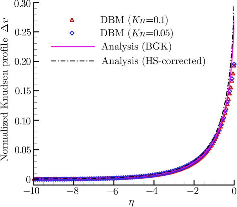
Fig. 

 | Fig. 5 Comparison of normalized Knudsen profiles from DBM simulations and those from analysis. |
Taking the TMAC (α) into consideration, the Maxwell-type boundary condition is adopted in the following simulation. The DBM simulation results with several different values of α are shown in Fig. 
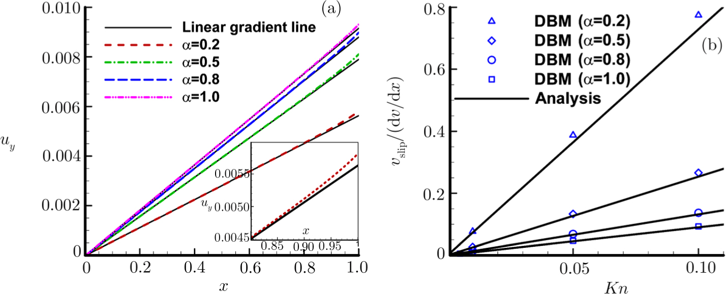 | Fig. 6 DBM simulation results for different values of α under Maxwell-type reflection boundary conditions. (a)  |
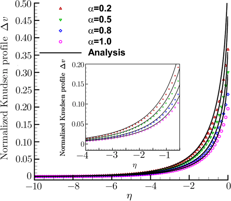 | Fig. 7 Comparison of normalized Knudsen profiles from DBM simulations with those from analysis for different values of α. A local enlargement is shown in the inset. |
3.2 Poiseuille Flow
31 ). Subsequently, Hadjiconstantinou[47] improved the model for a hard sphere gas by considering Knudsen layer effects. In his article, the viscosity-based mean free path, 


40 ) by the mean channel velocity 
Pressure driven gas flow, known as Poiseuille flow, in a microchannel is also very common in MEMS. In the slip-flow regime, the Navier–Stokes equations with slip boundary condition are applicable. Accurate second-order slip coefficients are of significantly since they directly determine the accuracy of the results given by Navier–Stokes equations.[47] The first second-order slip model was presented by Cercignani. Using the BGK approximation he obtained


It is clear that the pressure gradient and the viscosity coefficient vanish in the nondimensionalized 
The simulation results by DBM for different Knudsen numbers are shown in Fig. 
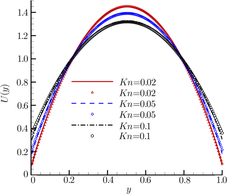 | Fig. 8 Comparison of velocity profiles between DBM results and analysis for different Knudsen numbers. Symbols represent the DBM results while lines represent the analytic ones. |
Considering the behaviours of velocity slip under various TMACs. Then the Maxwell-type boundary condition is used. It can be seen from Fig.
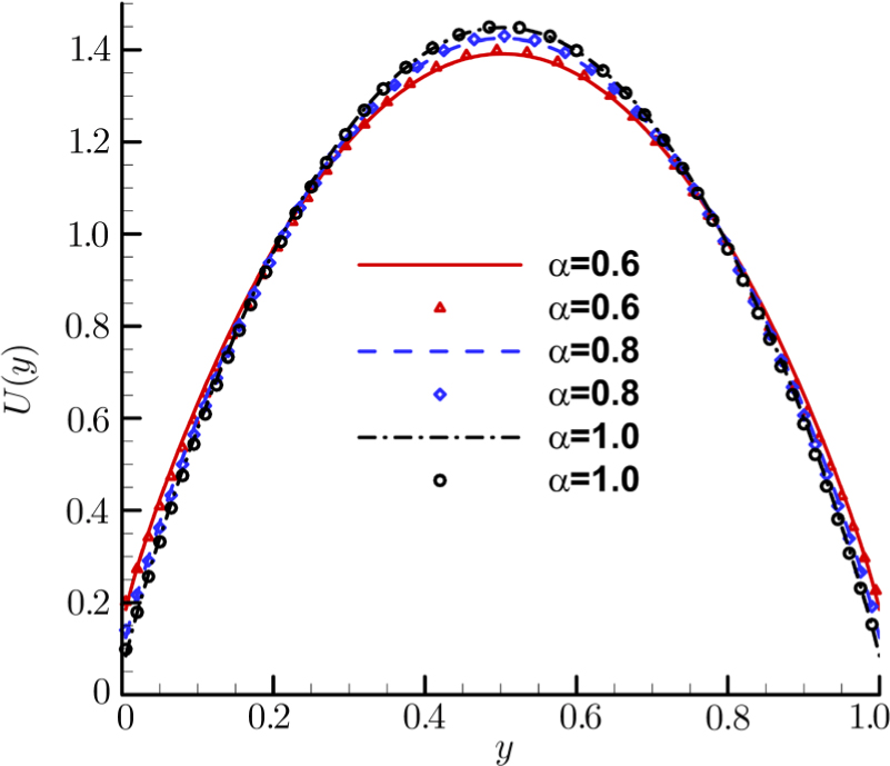 | Fig. 9 Comparison of velocity profiles between DBM results and analysis for different values of α. Symbols represent the DBM results while lines represent the analytic results. |
4 Conclusion
A discrete Boltzmann method with Maxwell-type boundary condition for slip flow is presented. The definition of Knudsen number is clarified for DBM. The relation between the Knudsen number based on hard sphere model and that based on BGK model is given. Two kinds of gas flows, including Couette flow and Poiseuille flow, are simulated to verify and validate the new model. The results show that the DBM with Maxwell-type can reasonably capture both the velocity slip and the flow characteristics in Kundsen layer under various Knudsen numbers and tangential momentum accommodation coefficients.
Reference
| [1] | |
| [2] | |
| [3] | |
| [4] | |
| [5] | |
| [6] | |
| [7] | |
| [8] | |
| [9] | |
| [10] | |
| [11] | |
| [12] | |
| [13] | |
| [14] | |
| [15] | |
| [16] | |
| [17] | |
| [18] | |
| [19] | |
| [20] | |
| [21] | |
| [22] | |
| [23] | |
| [24] | |
| [25] | |
| [26] | |
| [27] | |
| [28] | |
| [29] | |
| [30] | |
| [31] | |
| [32] | |
| [33] | |
| [34] | |
| [35] | |
| [36] | |
| [37] | |
| [38] | |
| [39] | |
| [40] | |
| [41] | |
| [42] | |
| [43] | |
| [44] | |
| [45] | |
| [46] | |
| [47] |