


A Study of ρ-ω Mixing in Resonance Chiral Theory
Cite this Article
Chen Yun-Hua, Yao De-Liang, Zheng Han-Qing. A Study of ρ-ω Mixing in Resonance Chiral Theory. Communications in Theoretical Physics, 2018, 69(1): 50 
Permissions
A Study of ρ-ω Mixing in Resonance Chiral Theory
† Corresponding author. E-mail:
Abstract
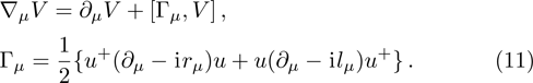
Abstract
The strong and electromagnetic corrections to ρ-ω mixing are calculated using an SU(2) version of resonance chiral theory up to next-to-leading orders in 


1 Introduction
The study of ρ-ω mixing is a very interesting subject in hadron physics both theoretically and experimentally. The inclusion of ρ-ω mixing effect is crucial for a good description of the pion vector form factor in 

The ρ-ω mixing amplitude was assumed to be a constant or momentum-independent in the early stage of previous studies.[4–5] The authors of Ref. [6] suspected the validity of the constant assumption and, based on a quark loop mechanism of ρ-ω mixing, they found that the mixing amplitude is significantly momentum-dependent. Since then, the use of various loop mechanisms for ρ-ω mixing is triggered in different models such as extended Nambu-Jona-Lasinio (NJL) model,[7] the global color model,[8] the hidden local symmetry model,[9–11] and the chiral constituent quark model.[12–13]
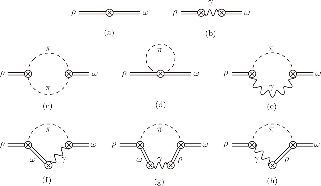
In this work, we aim at studying ρ-ω mixing in a model independent way by invoking Resonance Chiral Theory (RχT).[14] It provides a reliable tool to study physics in the intermediate energy region.[15–20] The tree-level calculation of ρ-ω mixing in the framework of RχT has been given in Refs. [21–22], however, the tree-level mixing amplitude turns out to be momentum-independent. In order to implement the momentum dependence, here we will calculate the one-loop contributions as shown in Fig. 


 | Fig. 1 Feynman diagrams contributing to ρ-ω mixing. |
We assess the impact of momentum-dependent ρ-ω mixing amplitude on the pion vector form factor by fitting to the experimental data extracted from the 


This paper is organized as follows. In Sec.
2 Generic Description of 
¶ and 


2 ) through
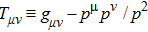
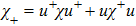
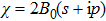
In the isospin basis 


In above the vector-current conservation has been used to eliminate the longitudinal part proportional to pμ. Furthermore, we have also neglected terms of 
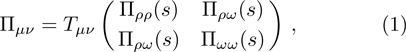
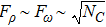
The ρ-ω mixing, i.e., mixing between the physical states of ρ0 and ω, is obtainable by introducing the following relation
Solving the above equation and neglecting higher-order terms of 

The two mixing parameters should be just different with each other slightly, see Ref. [35] for more details.
3 Calculations in Resonance Chiral Theory


1 are needed for a calculation in RχT up to NLO in 


1 will be calculated by using effective Lagrangians constructed in the framework of RχT.
In this section we will calculate the mixing amplitude 

3.1 Resonance Chiral Theory and Tree-Level Amplitudes


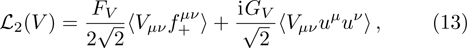
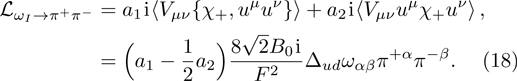
1 and the amplitude can be obtained by using the Lagrangian in Eq. (13 ):


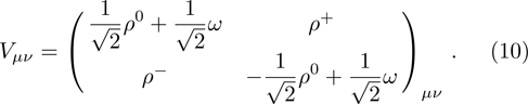
In RχT, the vector resonances are described in terms of antisymmetry tensor fields with the normalization


Besides, the covariant derivative and chiral connection are defined by
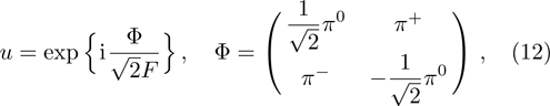
The Goldstone bosons originating from the spontaneous breaking of the 
In the isospin limit, the standard Lagrangian describing the interactions between 
Here 
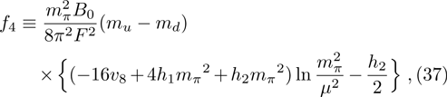
The LO isospin-breaking effect is introduced by the Lagrangian

With the above preparations, one is now able to calculate the tree amplitudes. The tree-level strong contribution, corresponding to diagram (a) in Fig.

3.2 Loop Contributions


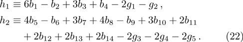
35 ) are a, f4, 


The relevant loop diagrams contributing up to our accuracy are shown in the second and third lines of Fig. 

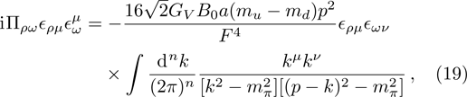
(i) Diagram (c): 
The vertex of 

For convenience, we define the combination 

(ii) Diagram (d): π-Tadpole Loop
According to the Lorentz, P and C invariances, the Lagrangian corresponding to the interaction of 
Note that the 

Furthermore, one can neglect the mass difference between the charged and neutral pions in the internal lines of loops, since the resultant difference is of higher orders beyond our consideration. As a result, the expanded form of Lagrangian (
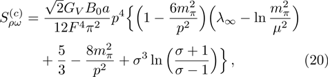
With the above Lagrangian, the π-tadpole contribution to the ρ-ω mixing can be derived:
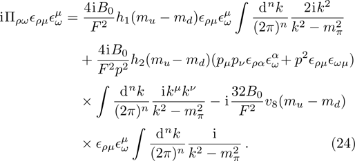
Eventually, the explicit expression of the strong structure function has the form of
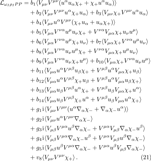
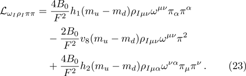
(iii) Diagrams (e)–(h): 
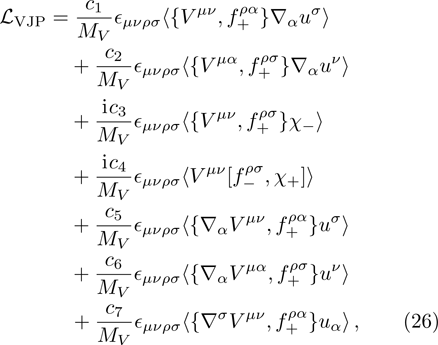
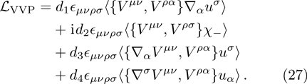
In the loop diagrams (e)–(h), there are two types of vertices. The coupling of vector meson (V) as well as vector external source (J) to pseudoscalar (P) is labeled by VJP vertex for short. The interaction of two vector mesons and one pseudoscalar is called VVP vertex. The operators of VJP type are given in Ref. [37]:
The involved couplings or their combinations can be estimated by matching the leading operator product expansion of 
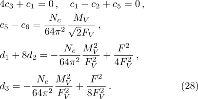
The mass of vectors in the chiral limit, MV, can be estimated by the mass of 
The loops diagrams (e)–(h) can be calculated simultanously if the effective vertices of 


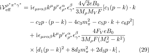
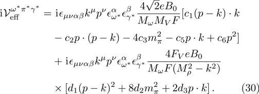
It should be stressed that there are two terms in each effective vertex. One corresponds to the case that the virtual photon is coupled to the VP system directly, while the other to the case that it is interacted through an intermediate vector meson. Note also that, throughout this work we only account for the corrections proportional either to 


With the help of the effective vertices, the 
The further calculation is straightforward but the result of the extracted electromagnetic structure function 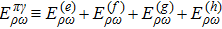

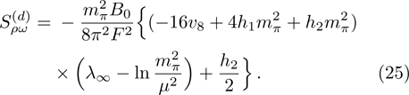
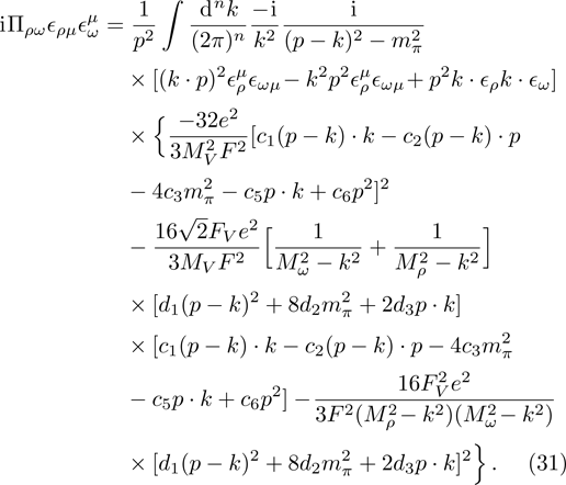
(iv) Counterterms and Renormalized Amplitude
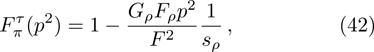
Up to now, the total contribution of ρ-ω mixing can be expressed as

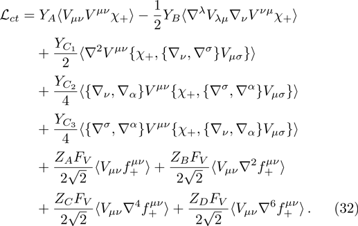
We adopt the 


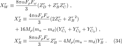
In summary, the UV-renormalized mixing amplitude reads
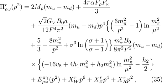

In our numerical computation, the scale μ will be set to Mρ and we use 
4 The Effect of 
3 ) now can be rewritten as


The mass and width of ρ meson are conventionally determined by fitting to the data of 

For the narrow-width resonance ω, we take 


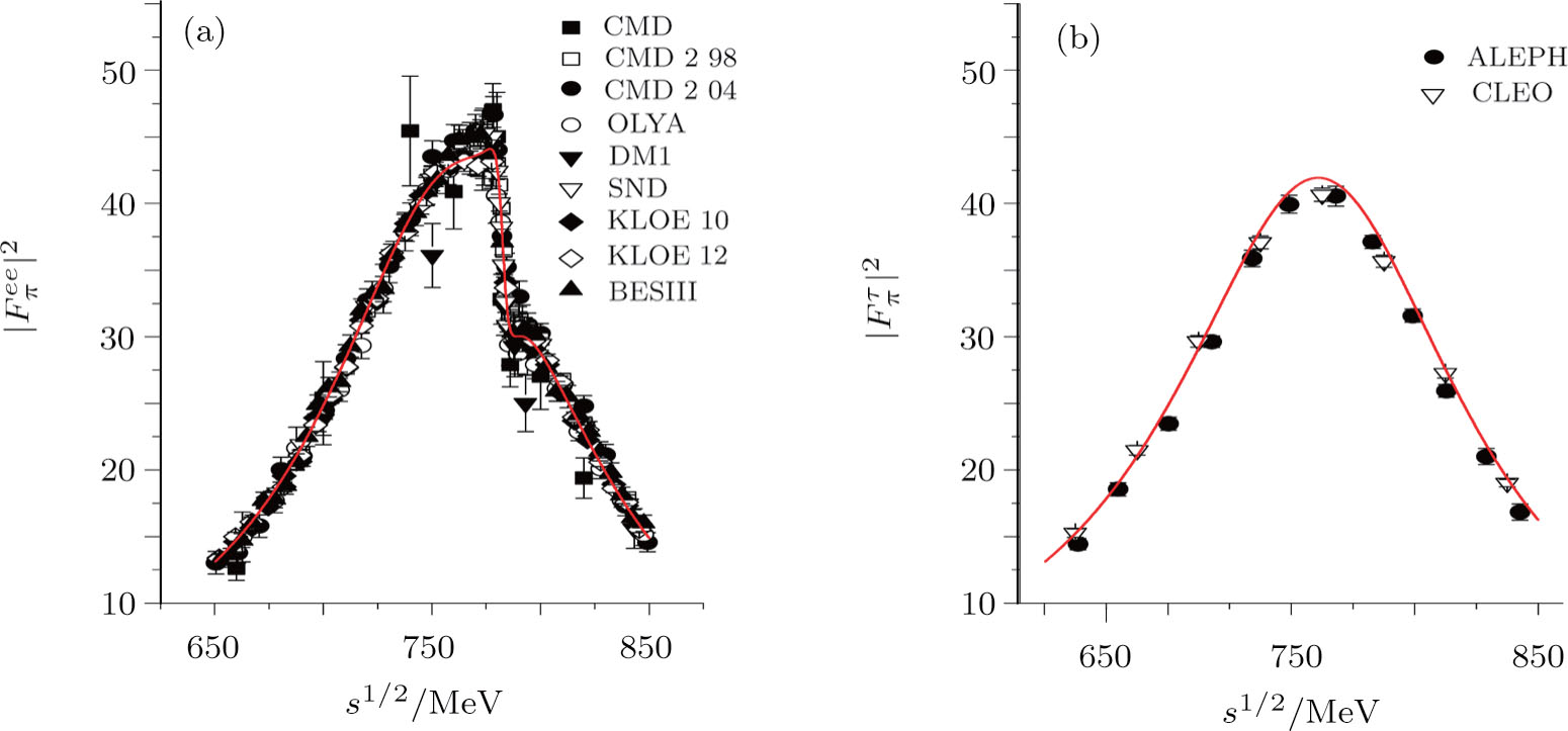
The experimental data considered in this work are the pion form factor 


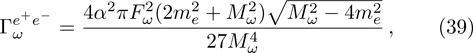
The Feynman amplitude for the process 
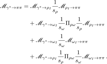
Here the fourth term corresponds to higher-order contribution of isospin breaking, e.g., proportional to 

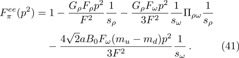
On the other hand, the expression of the pion form-factor in 

Our best-fitted parameters and the corresponding 

 | Fig. 2 (Color online) Fit results for the pion form factor in the    |
| Table 1
The fit results of the parameters. . |
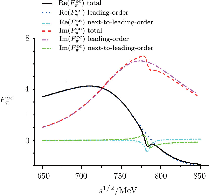
In Fig. 


 | Fig. 3 (Color online) The real and imaginary parts of the fitted form factor  |
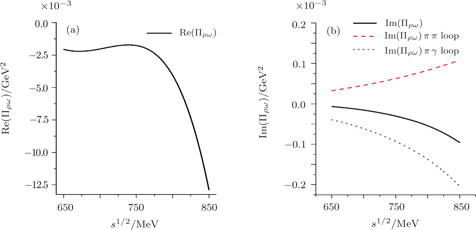
In Fig. 


 | Fig. 4 (Color online) The real part (a) and imaginary part (b) of the mixing amplitude    |
The values of 

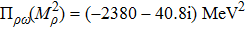


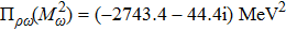

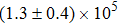
Using the central values of the fitted parameters in Table 
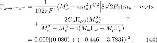
From Eq. (


5 Summary
We have analyzed the ρ-ω mixing within the framework of resonance chiral theory. Based on the effective Lagrangians constructed under the guidance of various symmetries, we calculate the ρ-ω mixing amplitude up to next-to-leading order in large 


Reference
| [1] | |
| [2] | |
| [3] | |
| [4] | |
| [5] | |
| [6] | |
| [7] | |
| [8] | |
| [9] | |
| [10] | |
| [11] | |
| [12] | |
| [13] | |
| [14] | |
| [15] | |
| [16] | |
| [17] | |
| [18] | |
| [19] | |
| [20] | |
| [21] | |
| [22] | |
| [23] | |
| [24] | |
| [25] | |
| [26] | |
| [27] | |
| [28] | |
| [29] | |
| [30] | |
| [31] | |
| [32] | |
| [33] | |
| [34] | |
| [35] | |
| [36] | |
| [37] | |
| [38] | |
| [39] | |
| [40] | |
| [41] | |
| [42] | |
| [43] | |
| [44] | |
| [45] | |
| [46] | |
| [47] | |
| [48] | |
| [49] |