


A Direct Algorithm Maple Package of One-Dimensional Optimal System for Group Invariant Solutions
Cite this Article
Zhang Lin, Han Zhong, Chen Yong. A Direct Algorithm Maple Package of One-Dimensional Optimal System for Group Invariant Solutions. Communications in Theoretical Physics, 2018, 69(1): 14 
Permissions
A Direct Algorithm Maple Package of One-Dimensional Optimal System for Group Invariant Solutions
† Corresponding author. E-mail:
Abstract
Abstract
To construct the one-dimensional optimal system of finite dimensional Lie algebra automatically, we develop a new Maple package One Optimal System. Meanwhile, we propose a new method to calculate the adjoint transformation matrix and find all the invariants of Lie algebra in spite of Killing form checking possible constraints of each classification. Besides, a new conception called invariance set is raised. Moreover, this Maple package is proved to be more efficiency and precise than before by applying it to some classic examples.
1 Introduction
Symmetry group theory has a priority to gain much concern in finding exact solutions of differential equations.[1–5] The theory is commonly applied to construct explicit solutions for integrable and non-integrable nonlinear equations. Based on the theory, an original nonlinear system of any given subgroup can be reduced to a system with fewer independent variables. The reduction of the variables is established on group invariant solutions. Since infinite subgroups always exist, which means the impossibility of finding all the group invariant solutions[6–9] to the given system, the classification[10–20] of symmetry subgroup is essentially important in solving the problem. Then to find those complete but inequivalent group-invariant solutions is expected. From now on, many systematic and effective method has formulated, and the concept of “optimal system” for group-invariant solutions is proposed to solve the problem.
People always find an optimal system of subalgebras instead of finding subgroups, which are equivalent. Ovsiannikov[21] initially uses the adjoint representation[22] of a Lie group on Lie algebra to classify group-invariant solutions and the method is developed by Olver, Winternitz, Zassenhaus, and Patera[23–24] afterwards. In particular, Olver[22] gave an ingenious method, which is more simple to calculate. For the one-dimensional optimal system, he successfully applied the method in the Korteweg-de Vries (KdV) equation and the heat equation. Later on, many new methods have appeared and the mechanization has been realized[25–31] through computer. The mechanized realization simplifies complicated manual computation efficiently. So to many important partial differential equations, this has always been paid substantial concentration.
The objective of this paper is to give a new Maple package for constructing the one-dimensional optimal system,[32] which can be more precise and common used. Here we propose a new symbolic computation algorithm and develop a Maple package named One Optimal System. For a given Lie algebra, it can find different cases of classification and the corresponding one-dimensional optimal system automatically. Compared to existing software packages, the improvement of the new software package is that it gets more precise result, which is equal to Olver’s result. What is more, it can be more common used in many important partial differential equations. So we have made a meaningful improvement in constructing the one-dimensional optimal system of finite dimensional Lie algebra.
This paper is arranged as follows. In sec.
2 Conceptions and Formulas
2.1 Optimal System
Suppose G is a Lie group. We define H as an optimal system of s-parameter subgroups, which are inequivalent to each other. It is a system of differential equations in p 

2.2 Adjoint Representation


2 ) means to apply the product of adjoint action 


Let 


2.3 Invariant
Suppose a real function ϕ. For all 


Then ϕ can be called an invariant. For any invariant, two vectors v and 

2.4 Classification Rules
We classify all the generators by assigning different values to the invariants. The rules of classification are as follows:
(i) Check every invariant’s degree. If we find the degree of an invariant is even, we can make it either 1 or 0. On the other hand, if the degree is odd, we can make it 1, −1 or 0.
(ii) For every invariant, it must be assigned either 1 or −1 (if degree is odd) firstly. And in each case, we must and just make only one invariant (marked as a flag invariant) either 1 or −1. Then the remaining invariants are assigned c at the same time. After that, we can make the flag invariant 0 with any other invariant assigned either 1 or −1. And the remaining invariants are assigned c at the same time.
(iii) Once an invariant is assigned 0, it cannot be assigned c any more. When all the invariants have been assigned either 1 or −1. The last case must be all the invariants are assigned 0.
2.5 Invariance Set
Suppose a nonzero vector 


3 Algorithms
We developed an automated software package One Optimal System on Maple versions 16 and above. The package is initialized by the command with One Optimal System. The software package is consisted of Lie_Bracket, commutator, lie_bracket, commutator_table, lie_bracket_cal, Linear Co, e_index, e0,eps, data_data, fun_set, n_deta, deta_pd, ep_solve, judge_s, special_e, aaa_solve, get_rid, get_solution, beauty_m, check_30, exper_30, check_fun, trans_ornot, excep_vv, deno_ax, beauty_c, and One Optimal functions. The main function is One Optimal:= proc(vs., consts). We will illustrate the whole software flow and introduce algorithm of fundamental steps with some important functions and parameters description.
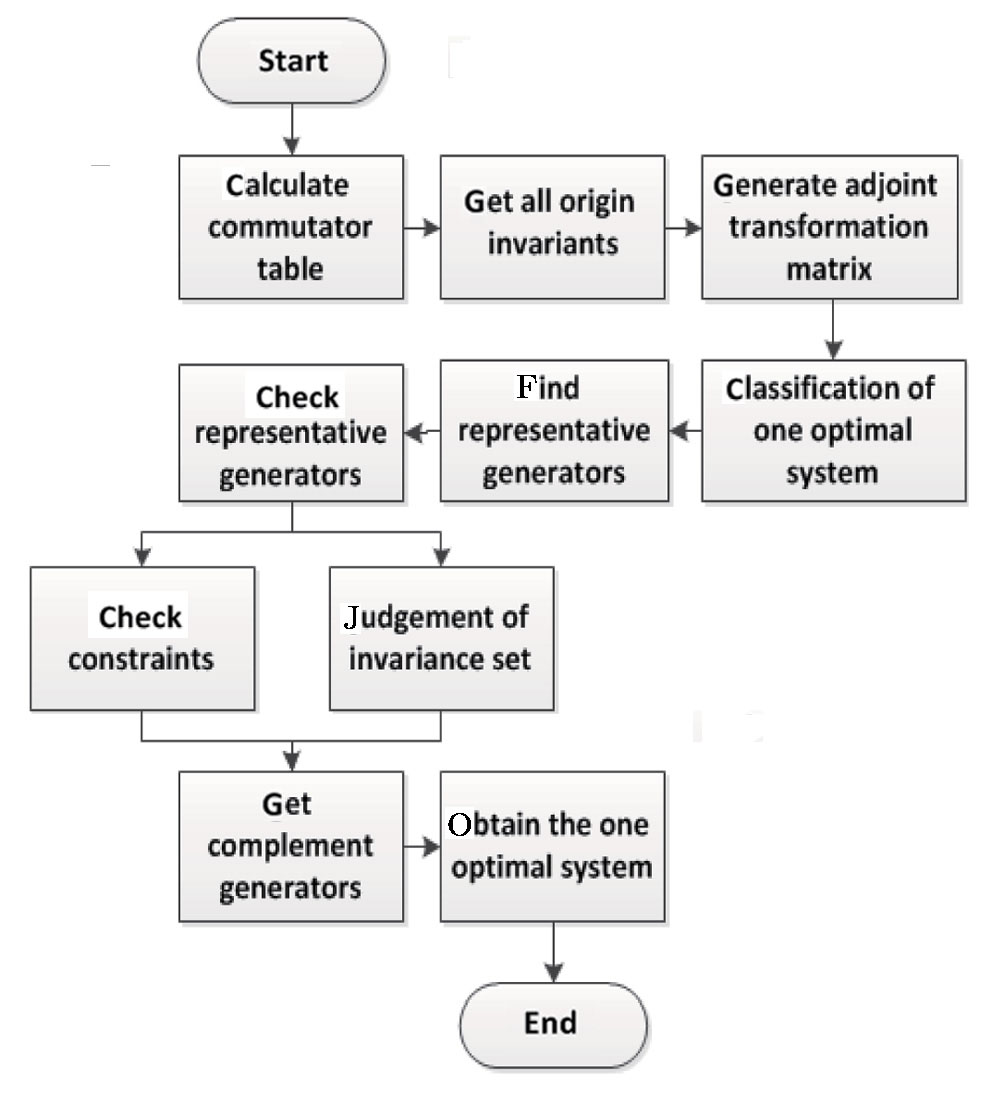
3.1 Overview of One Optimal System

9 ) with respect to ε and set ε = 0
Given the m-dimensional Lie algebra 

According to the definition of invariants (
By extracting the coefficients of bi, 


3.2 Generation of Adjoint Transformation Matrix
We can get the adjoint representation table by using formula (
Here we proposed a new algorithm to solve the problem. Without calculating formula (


Here is an example for KdV equation. Table 
| Table 1
The commutator table of KdV equation. . |
Compared with the old method, the new method is more sufficient and it is much easier for us to realize the calculating process through symbolic computation. Above all, the result is more accuracy than before.
Functions implementing this part as well as some important parameters are in Table
| Table 2
Functions and parameters of the One Optimal System. . |
3.3 Classification of One Optimal System
After we get all the invariants, we can classify each case of one-dimensional optimal system according to classification rules (details in Table 3).

(i) We assume invariant1 and invariant2 are origin invariants and initialize a current invariant set to put them in. For every cases, we assign exact value to the invariants in the current invariants set according to classification rules.
(ii) When there is no invariant assigned c, we substitute the case constraints into the differential equation to find if new invariants (assuming invariant3 and invariant4 represents new invariants in each case) exists. If all the invariants in the current set are not assigned 0, we should make all new invariants c. On the other hand, if all the invariants in the current set are assigned 0, we can add the new invariants into the current invariants set and assign exact value to them according to classification rules.
(iii) What we should notice is the new invariants are not constant if they are not added to the current set. The new invariants’ expression depend on the differential equation, which are substituted different case constraints.
(iv) The last column of Table
| Table 3
Different cases of classification for an optimal system. . |
Functions implementing this part as well as some important parameters are described in Table
| Table 4
Functions and parameters of the One Optimal System. . |
3.4 Find the Representative Generator
6 .
(i) Find a representative generator
For each case, we must choose a representative generator and it is better to be as simple as possible. For this intention, we solve case constraint firstly. Then we assume each ai showing in the numerator of the solution to be 0, except the one showing up in the denominator as well. And the one in the denominator should be assigned either 1 or −1, determined by another constraint (expressions like 
(ii) Check the representative generator
By solving Eq. (
(a) Exists expressions like 
(b) Exists denominator ai.
If so, this will make the chosen representative generator not complete. That means it can not represent the whole generators of this case. Then we should find another representative generator to complement the chosen one.

| Table 5
Two examples of the first situation. . |

(i) If the same constraint also exists in the case constraints, we do not need to find another generator as the constraints exist originally in this case.
(ii) Solution1 is for the case constraint and solution2 is for Eq. (
 | Fig. 1 Software flow diagram of the One Optimal System. |

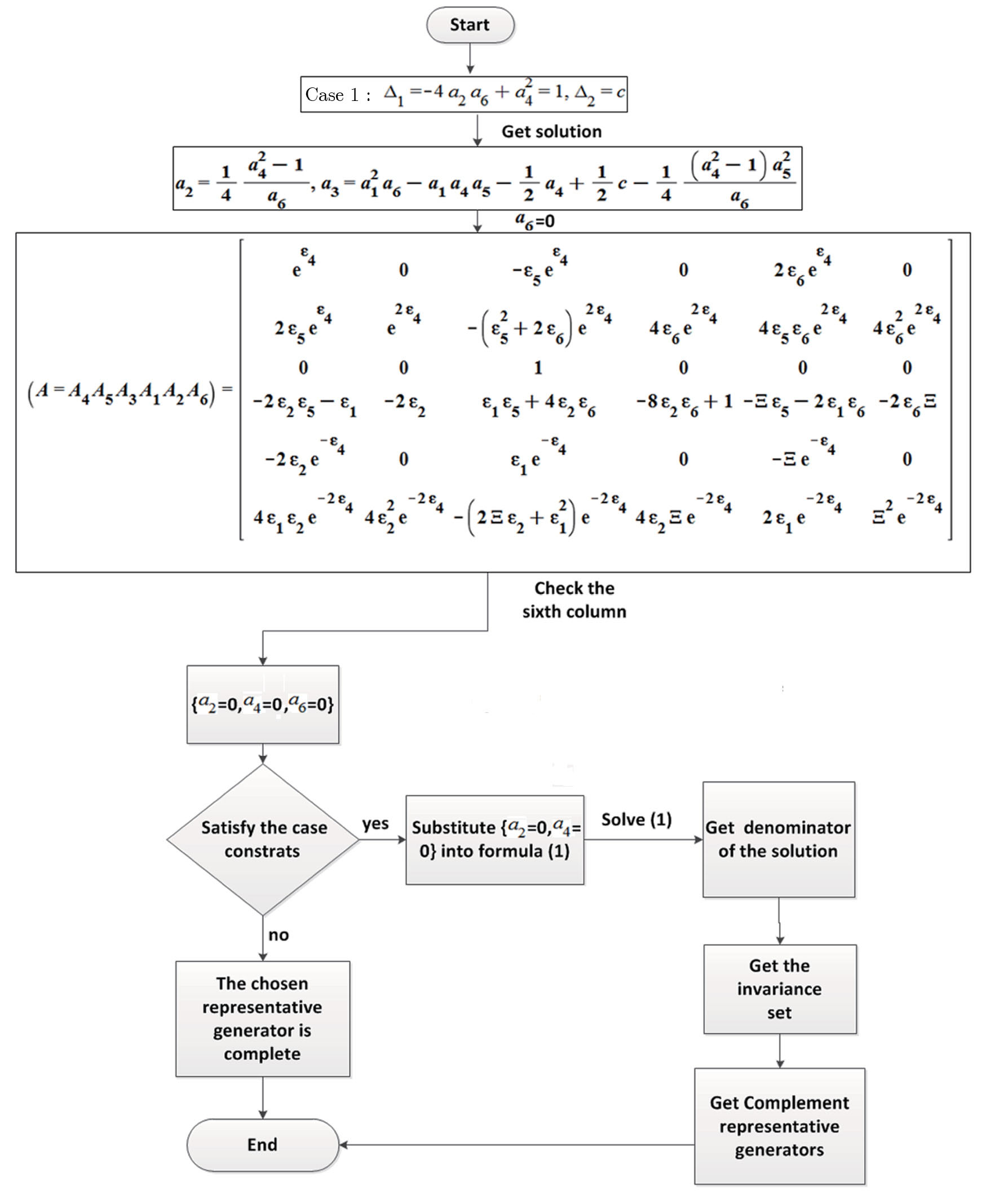
For this situation, it is related to the invariance set and we have a check method in Fig. 

 | Fig. 2 Software flow diagram of situation 2. |
If we get the invariance set, we can classify two cases as follows:
(i) Make all the variants 0 in the invariance set.
(ii) Make not all the variants 0 in the invariance set.
Then we can get two new representative generators. Through the two steps above, we can find the representative generator in every cases, but there is still a special situation we should also take a consideration. Take KdV equation for example. When we find the representative generators under the case constraints 

| Table 6
Functions and parameters of the One Optimal System. . |
4 Examples
According to the previous software package One Optimal,[33] which generates one-dimensional optimal system of finite dimensional Lie Algebra, the result has to adjust the coefficients containing ε, which is uncertainty to give a complete classification. This uncertainty makes problems that some of the representative generators of the one-dimensional optimal system are absent or belong to the same case. The new software package One Optimal System can overcome this problem by giving a direct classification, whose answer is equal to Olver’a result. In this chapter, we apply it to many important equations to check its effectiveness and correctness.
4.1 KdV (Korteweg-de Vries) Equation
7 is just the same as our answer.

—Inputs:


—Outputs:
The commutator table is as Table
| Table 7
The commutator table of KdV equation. . |
The origin invariants are: 
The cases discussed: 
The Optimal System is: 
According to Olver,[22] the one-dimensional optimal system of KdV Equation is
4.2 Heat Equation

—Inputs:


—Outputs:
The commutator table is as Table
| Table 8
The commutator table of heat equation. . |
The origin invariants are: 


The Optimal System is: 
According to Olver,[22] the one-dimensional optimal system of Heat Equation is

We can see (a) (c1) (c2) (d) is different from our answer. However, we can get these equivalent relationship as follows through the adjoint representative matrix A action in formula (

Thus, we get the equivalent answer of Heat Equation to Olver.
4.3 NS (Navier-Stokes) Equation


—Inputs:


—Outputs:
The commutator table is as Table
| Table 9
The commutator table of NS equation. . |
The origin invariants are: 
The cases discussed: 


4.4 ZK (Zakharove-Kuznetsov) Equation

—Inputs:


—Outputs:
The commutator table is as Table
| Table 10
The commutator table of ZK equation. . |
The origin invariants are: 
The cases discussed: 


The Optimal System is: 
5 Conclusions
Group invariant solutions have been used to describe general solutions to PDE systems. They can be illustrated by the invariance of PDE symmetry group. We need to find group invariant solutions due to the existence of infinite different symmetry groups. To classify invariant solutions in Lie algebra, we propose a new Maple package called One Optimal System. This has a significant meaning in the mathematics mechanization and machine learning. The mechanized realization efficiently make complicated manual computation much more simple. Especially, to many important partial differential equations, many researchers have paid substantial concentration to the theme. Compared with the previous software package,[33] this new software package is obviously more efficient than the previous one, which costs less time in operation. And we can get a perfect result that is precisely consistent with Olver’s result. And the algorithm of the new software package is more direct and programming than the previous one without many manual settings. Furthermore, the algorithm structure can be used to r-parameter 
We realize calculation process of the one-dimensional optimal system by developing One Optimal System software package, which is demonstrated effective, precise and systemic. This is proved to simplify the manual computation significantly and has made a contribution to mathematics mechanization. To achieve more pervasive mechanized application of this method, we will devote to developing new software package of r-parameter 
Reference
| [1] | |
| [2] | |
| [3] | |
| [4] | |
| [5] | |
| [6] | |
| [7] | |
| [8] | |
| [9] | |
| [10] | |
| [11] | |
| [12] | |
| [13] | |
| [14] | |
| [15] | |
| [16] | |
| [17] | |
| [18] | |
| [19] | |
| [20] | |
| [21] | |
| [22] | |
| [23] | |
| [24] | |
| [25] | |
| [26] | |
| [27] | |
| [28] | |
| [29] | |
| [30] | |
| [31] | |
| [32] | |
| [33] |